
The Spinozan Trader

A Geometric Critique of Strategies, Signals, and Evidence
Expanded reference edition · September 2026
A book by Kutty Stauder
The Spinozan Trader
A Geometric Critique of Strategies, Signals, and Evidence
Definitions, conditional proofs, counterexamples, historical research, and reproducible tests. Mathematical properties do not establish market profitability; evidence is labeled by its actual scope.
Kutty Stauder
Expanded reference edition · September 2026
Copyright © 2026 Kutty Stauder.
All rights reserved.
Philosophical inspiration: Baruch Spinoza. Contemporary prose and applications are by the author, not quotations from Spinoza unless expressly identified.
kuttystauder.com/books
How to Use This Book
A screen can contain twenty indicators and only one idea. The lines have different colors, the names come from different decades, and the trader feels surrounded by confirmation. Yet each line may be another transformation of the same recent prices. The screen has multiplied the appearance of evidence faster than it has multiplied evidence itself.
This book asks a harder question than whether an indicator is good. Good for what decision, in which market, over what horizon, using what information, at what cost, and compared with what alternative? A moving average can reduce the complexity of a decision without predicting a return. A volatility estimate can improve position sizing without forecasting direction. An execution algorithm can save money while having no view of tomorrow's price. A pattern can predict a conditional distribution and still fail to pay its spread.
The geometric method gives these distinctions a durable form. Definitions prevent an attractive word from doing the work of a calculation. Assumptions disclose the world in which an argument holds. Propositions state results narrowly enough to be demonstrated. Counterexamples expose conclusions that outrun their premises. Historical studies then confront the premises with a world that does not owe them continued truth.
Choose a reading route
On a first reading, take the method of proof, definitions, expectancy, sizing, and information together. Then read The Calculus of Usefulness. The line-by-line proof example and symbol guide explain the notation without assuming prior mathematical training. You can follow the prose and worked examples first, returning to a demonstration when you want to inspect its assumptions.
Choose the route that matches the decision you want to make:
| Your question | Read next | Produce before moving on |
|---|---|---|
| How do I specify my first systematic rule? | Where edge comes from, operation, and if the purchase is a challenge prop firms | A completed strategy worksheet that names the supposed payer, and a paper ledger |
| Where does a trading edge come from? | Edge chapter, usefulness, market making | Which of the named families, if any, your rule could access |
| How do prop-firm challenges work? | Prop firms, risk, livelihood | A written knockout sheet; passing is not expectancy |
| Which popular systems are being sold to me? | Atlas, the linked proofs, laboratory results | Each system's actual object: recoding, path constraint, or untested lore |
| Can I just watch candles and be successful over time? | Watching candles, livelihood | Which study, sample, exit, and cost you are borrowing; none is a discretionary livelihood |
| What is anchored VWAP, exactly? | The anchored VWAP, execution | A written object, volume, anchor clock, and role: benchmark, description, or trigger |
| Can I algo-trade like Jim Simons / Renaissance? | Algorithmic trading and its myths, edge | Which Renaissance book; Medallion is not RIEF and not a 13F copy |
| Is the COT report useful? Intraday or swing? | Commitments of Traders, futures | Tuesday snapshot, Friday 15:30; not an intraday increment; swing only after the print |
| Which tools on my chart do useful work? | Atlas, the relevant indicator chapter, then execution | Each tool's input, decision role, and a comparison with it removed |
| Does a backtest establish an edge? | Data, inference, laboratory protocol, results | A list of what was tested, what was selected, and what remains uncertain |
| Why can a “losing” rule still grow money, or a “winning” table still fail? | Murky backtesting, monthly results, opening-drive, random controls | Which meaning of lose you are using: expectancy, benchmark, path, or convention |
| How does the intraday ORB research translate into a test? | Closing ORB study, then operation | Separate specifications for stocks and futures; no transfer of return claims |
| How did the monthly SPY/cash filter behave? | Monthly construction, results | An investment-contrast worksheet; not the book's first trading method |
| How should I revise an existing process? | Blueprints, worked cases, exercises | A dated change proposal and a rule for rejecting it |
| What did the Turtle traders actually do? | Turtle chapter, then risk | A written unit, stop, and correlation-cap sheet; no transfer of Faith's 80% figure |
| How do I write a risk plan? | Risk management, sizing, operation | A completed risk worksheet with heat, gap, and pause rules |
| I trade forex or futures. Where could a repeatable edge come from? | Anatomy of a repeatable edge, instruments, edge chapter | A named payer, a net margin after costs, and the contract arithmetic that decides whether the size is even available |
| Which forex and futures strategies have public evidence? | Trend, carry, currencies, commodities, time and flow, public records | Each claim's sample, cost treatment, and status: gross or net, in sample, out of sample, or live |
| How do I test a published strategy, and how would I run the six-month momentum rule? | A paper examined, with momentum and inference | A written specification, a cost model, the months needed to see the edge, and a retirement rule |
| What exactly would I trade, and when would I stop? | Blueprints, operation, edge factory | A written specification with a sizing formula, a cost limit, and a retirement rule fixed in advance |
The historical survey supplies context. The indicator and strategy chapters are a reference: read the family you need rather than treating every formula as a prerequisite to a first experiment.
Keep the studies separate
Several kinds of evidence appear in this book. This map prevents a favorable number from becoming a claim about a different strategy.
| Construction | Evidence in this edition | What the reader can conclude |
|---|---|---|
| Edge taxonomy | Geometric identities EG1–EG3; edge chapter | Recodings of H are not a distinct payer; a challenge fee is not an expectancy proof |
| Prop-firm evaluations | Dated official rules plus PF1–PF3; prop firms | Passing, underlying expectancy, and payout are different objects; no industry pass rate |
| Random-rule SPY controls | Frozen coin-flip and shuffled channel, same tape as the laboratory; results | These random policies lost the full sample to buy-and-hold; a slice can still beat a named rule |
| Candlestick / “price action” rules | Sourced tests from 1975–2012 Japan and U.S. names, 5-minute DJIA, Taiwan windows, and 1973–1994 FX head-and-shoulders; watching candles | No inspected study follows discretionary candle-watchers as a school; isolated favorable tables depend on the exit and do not establish a livelihood |
| Anchored VWAP | Geometry V4–V8, Berkowitz–Logue–Noser 1988, TradingView formula, Shannon’s public definition; complete reference | A declared average of a declared history; no inspected journal test of reclaim or fade as a livelihood |
| Algorithmic trading / “like Simons” | ADV four-family split, 13F rule, Zuckerman/Cornell table as journalism, 2020 Medallion-versus-outside-fund year; myths | Automation is not an edge; Medallion is not a retail experiment; RIEF is the same firm’s other book |
| Commitments of Traders | CFTC clock and classifications, N3–N6, Sanders–Irwin–Merrin and energy Granger tests; COT | A Tuesday book released Friday; not an intraday signal; inspected panels find little lead from positions to returns |
| Monthly SPY/cash filter | The book's retrospective simulation; full protocol and results | An investment-contrast risk tradeoff, with substantial benchmark shortfalls; not the first trading method |
| Daily SPY indicator rules | Thirteen constructions under common assumptions; comparison | How these exact rules differ in exposure, return, drawdown, and costs |
| Stock ORB with daily RVOL ranking | An externally reported 2016–2023 study; stock section | A promising published claim requiring independent replication |
| Fixed-basket FAANG ORB | This edition’s long/short 2016–2023 test and separate 2024–2026 extension; opening-range study | Outcomes for five retrospectively selected survivors under declared costs and data restrictions |
| Long/short NQ ORB | Two limited 2026 public-data replays; pilot | Exploratory outcomes with unresolved contract and execution limitations |
| Donchian-gated SPY opening-drive | This edition's daily analogue, 1994–July 2026; closing study | A failed declared-edge test; not a 5-minute stock ORB and not the Turtle system |
| Cross-sectional factors and portfolios | Defined research factors and allocation identities; factors, portfolios | Investment-contrast literature and mathematics, not a recommended trading book |
| Other strategy templates | Conditional mathematics and identified family literature; blueprints | Questions and specifications for research, not new backtested recommendations |
| Turtle / Donchian futures system | Faith's published rules plus later trend-following papers; Turtle chapter | A complete-system specification and long-horizon family evidence, not a reconstructed Turtle book |
| Risk plan | Geometric identities and worksheets; risk management | Explicit heat, caps, and gap rules; not a source of expected profit |
| Forex and futures strategy families | Sourced public studies, with no backtest run by this edition; anatomy of an edge to blueprints | Every figure belongs to someone else's sample, labelled gross or net of costs and in sample or live; the blueprints are specifications rather than tested results |
| Carry and insurance-like premia | The cross-asset carry literature, its drawdown record, and dated crashes; CY1–CY4, carry | A real premium with a measured negative skew; a smooth sample is evidence about the states it did not contain |
| Contests and long public records | Operator-published standings and managers' own factsheets; PR1–PR2, public records | Self-reported and unaudited, sometimes restated across different accounts and leverage levels |
The daily SPY laboratory uses February 1994 onward; the monthly study has its own start and initialization. Compare each strategy with the benchmarks calculated inside its own experiment. Dollar profit from one fixed futures contract, a stock portfolio's cumulative percentage return, and a fund strategy's annual growth rate are not a common ranking scale.
The evidence key
A definition is a convention used in this edition. Different software can implement the same named indicator differently. The edition states lookback, smoothing, seed, equality rule, and timing where these affect a result.
A proposition is an original demonstration in this book unless a source is explicitly credited. The first twenty-nine propositions retain their numbering from the shorter edition. Later propositions have stable family identifiers, such as F1 for filters. A label is a way to find an argument, not a claim that the author has discovered a previously unknown theorem.
An empirical finding reports an identified study or this edition's own calculation. Dates, market, comparison, and limitations travel with the finding. Results from a diversified futures study are not silently transferred to a single stock ETF. An intraday effect is not treated as evidence for a monthly rule.
A counterexample disproves a universal statement by constructing a permitted case in which it fails. It does not establish the frequency of that case in actual markets. One steadily rising price path disproves “RSI above 70 must be followed by a decline.” It does not establish that an RSI-based strategy always loses.
A working hypothesis is a proposition about markets that remains to be evaluated. A usefulness verdict identifies which roles are supported by the argument, which need empirical evidence, and which stronger claims have failed. The verdict can be favorable about measurement and unfavorable about a promotional promise at the same time.
Terms to keep beside the results
| Term | Meaning in use |
|---|---|
| Expected value or expectancy | Mean payoff under a stated probability model; a sample average estimates it |
| Net profit | Profit after the costs included in that calculation; check which costs were omitted |
| CAGR | The constant annual compound rate connecting starting and ending wealth, under the stated cash-flow convention |
| Drawdown | Decline from a previous equity peak; daily-close measurement can miss intraday losses |
| Basis point (bp) | 0.01 percentage point; 5 bp of $10,000 is $5 |
| One risk unit (R) | The strategy's defined initial risk amount; it is not a guarantee of maximum realized loss |
| Out-of-sample evaluation | Evaluation on observations excluded from the specified fitting process; a repeatedly inspected holdout is no longer fresh |
| Trading edge | A claimed favorable net decision advantage against a stated alternative, requiring evidence beyond the indicator formula |
Scope and date
The historical spine begins in the 1960s and follows the principal families into contemporary electronic and data-intensive trading. Earlier charting traditions appear where they explain an ancestor. This is a broad reference, not an enumeration of every proprietary strategy, every local-market convention, or every indicator variant. Contemporary source notes are dated to the September 2026 edition; exchange rules and product details must be rechecked when a strategy is implemented.
The monthly SPY study, daily indicator laboratory, random-rule controls, and closing ORB study each retain their own assumptions and evidence status. The forex and futures part, chapters 45 to 56, is a review of publicly documented strategy families and contract mechanics rather than an experiment of this edition's own: it reports other people's samples and states that no backtest was run here, so its blueprints are specifications to be tested rather than results to be trusted. The monthly filter and the factor and portfolio chapters are investment contrasts: they are retained as honest evidence, not as the first trading route. The downloadable companion contains protocols, code, tests, results, and input hashes. Reproduction requires the documented market inputs; the companion does not redistribute raw vendor data.
A reader's first experiment
Take one proposed trade. Write five sentences before looking for another indicator:
- The instrument and exposure I would hold are these.
- The information available before my order is this.
- The mechanism that could pay me is this.
- The observation that would make me reject the mechanism is this.
- After costs and adverse execution, the loss I can survive is this.
If the third sentence is merely the name of an indicator, the argument has not begun. Name the family in the edge chapter, or admit that none applies. If the fourth sentence is impossible to write, the idea may be protected from evidence. If the fifth sentence depends on a fill the market has not promised, the account is carrying an assumption the trader has not acknowledged.
Carry those five sentences into the strategy worksheet when you are ready to make the experiment executable. A good trading book should leave the reader harder to deceive, including by the book itself.
Chapter 1
The Method of Proof
The trader enters a world of numbers and too often leaves it with a superstition. A pattern becomes a promise. A winning month becomes a theory. A loss becomes an insult. The account records a result, but the mind supplies a story about what the result must mean.
The geometric method begins elsewhere. It asks what the terms mean, which premises are being granted, and what follows from them. It does not reward a conclusion for being forceful. The trader who writes “therefore” must show the bridge.
This book uses the architecture familiar from Euclid and Spinoza: definitions, common assumptions, propositions, demonstrations, corollaries, and explanatory notes. It borrows a discipline of reasoning, not the subject matter of Euclidean geometry. A market is not a triangle, and an empirical premise does not become self-evident because it has been called an axiom.
We will establish truths about the arithmetic of trading: expectancy, costs, compounding, drawdowns, position sizing, information, and the conditions of long-run growth. These results are conditional on explicit models. We will then construct a particular method and examine its historical record. The distinction between a theorem and a tested hypothesis is the spine of the book.
Three kinds of statement
A definition fixes how a term is used. Defining an edge as positive expected profit does not demonstrate that a trader possesses one. Defining a trend as a price above an average does not demonstrate that the price will continue upward.
A deduction establishes a conclusion from premises. If a position loses half its value, it must double to recover. Nothing about tomorrow's market is needed to prove that statement. If a proposed argument requires tomorrow's distribution, that distribution must appear among its premises.
An empirical claim concerns what occurred or is likely to occur in the world. Whether a trend filter has reduced drawdowns after realistic costs is such a claim. Data, execution conventions, alternative explanations, and uncertainty belong beside it. A historical result must carry its dates.
The error we are trying to remove is the quiet substitution of one category for another. “I can calculate the optimal stake if I know the odds” becomes “I know the optimal stake.” “This rule succeeded in these observations” becomes “this rule works.” “Every event has causes” becomes “I can predict the next event.” Each substitution removes the most difficult premise from view.
Read a proof as a short argument
You do not need to know geometry to begin. The Euclidean method used here means stating the starting points and showing each step to a conclusion. It is a way to organize an argument. The word proof does not make an assumption about markets true.
| Part of the argument | Plain-language question |
|---|---|
| Definition | What exactly does this word or symbol mean here? |
| Assumption or postulate | What are we granting for the argument, and could it fail in practice? |
| Proposition | What precise statement are we trying to establish? |
| Proof or demonstration | How does each step follow from the starting points or an earlier result? |
| Corollary | What further conclusion follows directly? |
| Scholium | What explanatory note helps me interpret or use the result? |
| Counterexample | Can one allowed case show that an “always” claim is false? |
| Q.E.D. | The argument is finished; the letters abbreviate “which was to be demonstrated” |
A proof translated line by line
Take the first proposition in the next group: net profit equals gross profit less costs. The letters are temporary names for amounts. Let G mean gross profit, C mean costs, and X mean net profit, all measured in dollars.
X = G − C reads: “Net profit equals gross profit minus costs.” If gross profit is $100 and costs are $7, net profit is $93. The letters let the same statement work for other amounts without rewriting the sentence.
Now consider possible trades rather than one completed trade. E[X] reads “the expected value of X”: the probability-weighted mean of its possible outcomes under the assumed model. It is not a promise about the next trade, and the letter E is not another amount being multiplied by X.
E[X] = E[G] − E[C] reads: “Expected net profit equals expected gross profit minus expected costs.” Taking a probability-weighted average preserves subtraction, provided the averages exist. That is the demonstration. It remains valid when profitable trades and costly trades tend to occur together; independence is not required for this accounting identity.
What has been proved? How the quantities relate. What remains unknown? The actual future distribution of gross profits and costs. The formula cannot supply those inputs. This separation is the habit to carry into the rest of the book.
Follow the labels without memorizing them
“Proposition 3” is an address, not the third step of a trading system. “Depends on D4, A2” sends you to Definition 4 and Assumption 2 in the foundational definitions. Read those starting points before deciding whether the conclusion applies to your account.
Later propositions use family labels: U1 is the first usefulness proposition, F1 the first filter proposition, and ORB1 the first opening-range proposition. Their numbers identify arguments, not confidence scores or recommended parameter values. The linked index lists every proposition.
Some letters recur in different chapters. “Definition D1” and “Proposition D1” are different addresses; the latter belongs to the data family. The same distinction applies to an assumption labeled A1 and a factor proposition labeled A1. Local headings and the index resolve the meaning. A range such as D2–D3 means both definitions, not a subtraction.
When a proof uses unfamiliar mathematics, first read its proposition, assumptions, example, and explanatory note. The symbol guide will help you return to the formal steps. Skipping those steps is a reading choice, not independent verification of the proof.
The Spinozan connection
Spinoza distinguishes activity from passivity through adequate causation and adequate ideas (Ethics III, definitions 1–3 and proposition 1). He describes conatus as a thing's striving to persevere (III, propositions 6–7). Those concepts suggest a useful orientation: preserve the capacity to act, examine the causes of your conduct, and do not confuse the intensity of an affect with evidence.
They do not establish that prices have a biological desire to persist, that every frightened person makes a bad trade, or that a trading loss proves inadequate understanding. A well-specified strategy can lose on an outcome its model allows. A poor strategy can win by chance. The mathematical distinctions below prevent the philosophy from becoming another instrument of self-deception.
A statistical regularity can be useful before its entire causal mechanism is known. A compelling causal story can be useless if the relevant effect is already reflected in price. The standard is explanatory honesty joined to observable performance, not a requirement that a finite trader comprehend the whole market.
What this edition promises
Forty-five chapters and one hundred thirty-nine propositions examine the principal trading families from the 1960s to the present. The original twenty-nine propositions establish the mathematical foundation; later demonstrations analyze indicators, strategies, execution, and inference. A fully specified equity/cash rule and a comparative indicator laboratory provide reproducible historical evidence, including costs and adverse comparisons. The atlas, worked cases, strategy blueprints, and operating protocol turn the arguments into a method of evaluation.
The aim is not a method that cannot lose. Proposition 23 explains why history cannot supply that guarantee. The aim is a method clear enough to execute, limited enough to survive mistakes, and explicit enough to be rejected when it fails its declared purpose.
To read geometrically is to ask of each page: What is defined? What is assumed? What has actually been shown? This is the first discipline of the Spinozan trader.
Chapter 2
Definitions and Assumptions
A letter stands in for a quantity so that an argument can cover many cases. Read its definition as an ordinary sentence before using the formula. Keep the units attached: a dollar amount, a share count, a probability, and a percentage return cannot be exchanged simply because each is written with one letter.
A guide to the symbols
Letters, time, and percentages
| Notation | Read it as | Example or caution |
|---|---|---|
| X | A trade outcome in the foundational model | X = −5 means a net loss of five stated monetary units |
| Vₜ or V_t | Portfolio value at time t | V₀ is starting value; Vₜ₋₁ is value one period earlier |
| t and n | A time label and a count | A period may be a minute, day, or month; the rule must say which |
| rₜ | Return during period t | rₜ = 0.05 means 5%, so 1+rₜ = 1.05 |
| p and 1−p | An event's probability and its complement | If p = 0.40, the complementary probability is 0.60 |
| w or f | A weight or fraction under its local definition | Use f = 0.01 when calculating with a 1% fraction |
| E[X] | Expected value of X | A model average over possible outcomes, not necessarily a historical sample mean |
| E[X | Hₜ] | Expected value of X given information Hₜ | The vertical bar means “given,” not division |
| f(x) | The value of a function at input x | A named calculation applied to x; not necessarily f times x |
The book uses both plain-text subscripts such as V_t and typographic ones such as Vₜ. They mean the same thing. A subscript labels an observation; it does not multiply the letter by the label. Parentheses in V_(t−1) group the time label “t minus one.”
A letter's meaning is local. H may mean a price high in one chapter, the account's previous peak in a drawdown calculation, or an information set in a probability argument. C may mean close, cost, or an option price. Read the accompanying definition rather than carrying a meaning from a previous chapter without checking it.
Operations and comparisons
| Symbol | Plain-language meaning |
|---|---|
| =, ≠ | Equals; does not equal |
| > < | Strictly greater than; strictly less than |
| ≥, ≤ | Greater than or equal to; less than or equal to |
| × or adjacent quantities | Multiply: pW means p × W |
| / or a fraction bar | Divide: a/b means a divided by b |
| ( ) and [ ] | Group the enclosed calculation, or identify a function's input |
| x², xⁿ | Powers: x² means x × x; xⁿ multiplies n copies when n is a positive integer |
| Σ | Add the indicated terms; Σxₜ might mean x₁+x₂+…+xₙ |
| ∏ | Multiply the indicated terms; ∏(1+rₜ) compounds the return factors |
| √x | Square root: the nonnegative number whose square is x, for x ≥ 0 |
| max, min | Largest or smallest of the specified values |
| |x| | Absolute value: distance from zero, so |−5| = 5 |
| ≈ | Approximately equal, often because of rounding |
In the absolute-value row, the bars surround a single quantity. That use differs from the “given” bar inside a conditional expectation. Context and the words beside the formula tell you which is intended.
Symbols used in the more mathematical chapters
Greek letters are names for quantities too. μ (mu) often denotes a mean; σ (sigma) a standard deviation; ρ (rho) a correlation; and ε (epsilon) an error or unexplained change. α (alpha) and β (beta) often label a regression intercept and exposure. Their specific meanings and units still come from the local model.
Var(X) measures dispersion around a mean. Cov(X,Y) measures how two quantities vary together. Δx means a change in x. A hat marks an estimate, and a star often marks a candidate optimum under the stated model. None of these decorations certifies that a fitted estimate will remain correct.
ln(x) is the natural logarithm. Its useful role here is to turn multiplication of positive wealth factors into addition: ln(ab)=ln(a)+ln(b). A derivative, written g′(f), describes the slope of g as f changes. The second derivative g″ describes how that slope changes. An integral, ∫, adds contributions over a continuous interval. The relevant chapters state the extra assumptions when using these tools; the plain-language conclusions and worked examples can be read first.
A symbol such as floor(x) rounds down to an integer, while ceil(x) rounds up. If a planned stop distance is 1.10 price units and a tick is 0.25, rounding the distance outward gives ceil(1.10/0.25) × 0.25 = 5 × 0.25 = 1.25. The rounding instruction changes the order level, not the certainty of its fill.
Definitions
D1. Price and information. A price is a quoted or executed exchange price at a specified time and venue. Let F_t denote information available to the strategy at decision time t. Price is not defined here as fair value, intention, or a complete equilibrium of human desires.
D2. Trade outcome. X is a trade's net profit or loss in specified monetary units, after the costs included in its model. A probability distribution for X describes a population of possible outcomes, not a verdict on one observed trade.
D3. Expectancy and edge. Expectancy is E[X], where the expectation exists. A positive-expectancy edge means E[X] > 0 under the relevant distribution. An estimate of edge is an estimate; it is not the distribution itself.
D4. Capital and return. V_t is marked portfolio equity after period t. With no external cash flows, its net return is r_t = V_t / V_(t−1) − 1. Positive equity is required wherever ratios or logarithms are used.
D5. Drawdown. Let H_t be the largest equity previously attained, including initial equity. Drawdown is d_t = 1 − V_t/H_t. Maximum drawdown is the largest d_t in a specified observation interval; a historical maximum is not a future loss limit.
D6. Practical ruin. Ruin means crossing a specified inability-to-continue threshold. Zero equity, a margin breach, and a personal minimum-capital threshold are different definitions and must not be interchanged.
D7. Position and exposure. An equity weight w is the fraction of portfolio value exposed to the equity instrument at a specified time. A rule restricting 0 ≤ w ≤ 1 prohibits shorting and portfolio leverage in this model. It does not remove the instrument's own market risk.
D8. Costs. Costs include modeled commissions, spread, slippage, financing, and other charges. A cost convention specifies whether a rate applies to traded notional or total capital. Taxes and inflation are separate unless explicitly included.
D9. Binary bet. A simplified bet wins net b units for each unit staked with probability p, or loses the stake with probability q = 1−p. A stake fraction f produces wealth factors 1+bf or 1−f. This model is not assumed to describe all market trades.
D10. Log growth. The expected log wealth increment of a strategy is E[ln(1+r)], when defined. For a binary bet, g(f) = p ln(1+bf) + q ln(1−f). Long-run compound growth and arithmetic expected profit are different objectives.
D11. Trading method. A method specifies instruments, data, observation times, signal, size, order timing, costs, and failure handling. A label such as trend following or buying strength is not yet a method.
D12. Empirical adequacy. In this book's practical vocabulary, empirical adequacy means that a claim fits stated evidence and survives relevant checks within a specified scope. This is a contemporary research standard, not an assertion that a backtest attains Spinoza's technical adequate idea.
Common assumptions
A1. Arithmetic and probability. Ordinary arithmetic, linearity of expectation, and probability identities apply where their quantities are defined. Results using variances or expected logarithms explicitly require those moments to exist.
A2. Accounting. External deposits and withdrawals are absent during the compounding examples. Dividends, fees, and corporate actions must be consistently included in the definition of portfolio return. Nothing is earned twice by changing notation.
A3. Positive wealth. Logarithmic results apply only while wealth factors remain strictly positive. The binary examples use b > 0 and 0 ≤ f < 1, with 0 < p < 1 unless a boundary is explicitly considered.
A4. Non-anticipation. Decisions may depend on F_t but not information that becomes available afterward. Knowing a final closing value generally means acting after that observation, not retroactively at the same price.
A5. Nonnegative modeled costs. The costs in comparisons are nonnegative, and the comparisons hold gross positions and outcomes fixed unless they say otherwise. Rebates and market-making economics require a different net-cost specification.
A6. Conditional repetition. Independence, identical distributions, and stable parameters are assumed only in propositions that explicitly invoke them. They are not general facts about financial markets.
A7. Admissible uncertainty. In the no-guarantee construction, both an adverse and a favorable next price move are compatible with the information already observed. No known contractual payoff or arbitrage eliminates that uncertainty for the directional position considered.
A8. Observation versus estimation. A historical record is finite. Its estimated probabilities and costs may differ from the future environment. Claims about future distributions require more than the identity of past observations.
How dependencies are read
“Depends on D4, A2” means that the conclusion relies on the definition of return and the absence of outside cash flows. It does not mean that a real account with deposits can be compared without adjustment. A proof is useful precisely because it exposes what changes when a premise changes.
The practical method later adds empirical hypotheses, designated H1–H3, and design choices, designated R1–R9. They are deliberately not added to the axioms as guaranteed properties of markets.
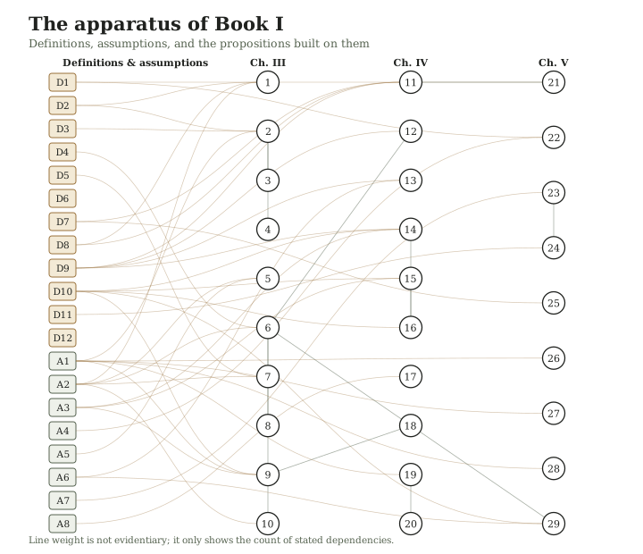
Figure 1. every line above is drawn from a real "Depends on" statement in chapters 3 through 5. The graph is generated directly from the manuscript, not hand-drawn, so it cannot drift from what the propositions actually cite.
Chapter 3
Expectancy and Compounding
Read each heading as the claim, the italic dependency line as its starting points, and the proof as the connecting argument. The worked examples translate the symbols into amounts. The proof-reading guide and symbol guide remain available whenever a letter or operation is unfamiliar.
Proposition 1Net profit is gross profit less cost.
Depends on D2, D8, A2.
Proof. Let G be the marked profit before the modeled costs C. By the accounting definition of net profit, X = G−C. Taking expectations where they exist gives E[X] = E[G]−E[C]. ∎
Scholium. A commission-free label does not establish C = 0. Spread and execution shortfall can remain. Equally, an expense already embedded in a fund return must not be deducted a second time. Define the ledger before discussing performance.
Proposition 2A two-class trade population has expectancy pW−(1−p)L−C.
Depends on D2–D3, A1; assumes exhaustive winning and losing classes with finite conditional mean payoffs.
Proof. Let p be the probability of a gross winning trade, W its conditional mean gross gain, and L the conditional mean magnitude of a gross losing trade. Assign any zero outcome consistently. The law of total expectation gives E[G] = pW+(1−p)(−L). Subtract expected cost C by Proposition 1. ∎
Example. At a 40% win rate, a $200 mean win, a $100 mean loss, and $5 expected cost, expectancy is $80−$60−$5 = $15 per trade. Those numbers define a hypothetical population. A trader must still establish whether observations justify using them.
Proposition 3Positive expectancy requires p > (L+C)/(W+L).
In words: the chance of a win must exceed the break-even fraction determined by average gains, losses, and costs. W is the average gross win, L the positive magnitude of the average gross loss, and C the expected cost per trade. This condition uses those specified inputs; it does not estimate them.
Depends on Proposition 2; assumes W+L > 0 and fixed W, L, C.
Proof. Positive expectancy means pW−L+pL−C > 0. Thus p(W+L) > L+C. Dividing by the positive denominator yields the stated condition. ∎
Corollary. Costs increase the break-even winning probability when other quantities remain fixed. They cannot be omitted because the strategy wins often.
Proposition 4Win rate alone does not determine profitability.
Depends on Proposition 2.
Proof by counterexample. Strategy A wins 90% of the time, gaining $1 on a win and losing $20 on a loss, with zero cost. Its expectancy is $0.90−$2 = −$1.10. Strategy B wins 40% of the time, gaining $3 and losing $1, also without cost. Its expectancy is $1.20−$0.60 = $0.60. The higher-win-rate strategy has negative expectancy and the lower-win-rate strategy has positive expectancy. Therefore win rate is insufficient. ∎
Scholium. An attractive hit rate may be purchased by occasional large losses. Look at payoff magnitude and tail behavior, not merely the frequency of being right.
Proposition 5Additional nonnegative costs cannot improve the same gross return path.
Depends on A2, A5; assumes comparable positive multiplicative wealth factors.
Proof. Write each gross wealth factor as a_t > 0. Let the two net factors be a_t−c_t and a_t−k_t with 0 ≤ c_t ≤ k_t < a_t. Each first factor is at least the second. Multiplying positive factors preserves the ordering. The wealth path with larger deductions has no larger terminal wealth. ∎
Limitation. This does not prove that low turnover always beats high turnover. A different trading rule may earn a different gross return. The proposition isolates costs, not strategy quality.
Proposition 6Capital compounds by multiplication.
In words: each percentage return acts on the capital then remaining. V₀ names the starting capital; Vₙ names capital after n periods. The product symbol ∏ below means to multiply all the intervening return factors.
Depends on D4, A2.
Proof. From D4, V_t = V_(t−1)(1+r_t). Repeated substitution gives V_n = V_0 × ∏(1+r_t), for t = 1 through n. ∎
Corollary. An arithmetic average of returns does not by itself specify terminal wealth. The complete sequence of wealth factors matters through their product. With no intervening flows and fixed factors, rearranging their order leaves the product unchanged, although the interim drawdown path changes.
Proposition 7Recovering a fractional drawdown d requires gain d/(1−d).
Depends on D5, A2; assumes 0 ≤ d < 1.
Proof. Equity after the loss is H(1−d). To recover H, a subsequent gain g must satisfy H(1−d)(1+g) = H. Dividing and rearranging gives g = 1/(1−d)−1 = d/(1−d). ∎
| Drawdown | Required recovery |
|---|---|
| 10% | 11.11% |
| 25% | 33.33% |
| 50% | 100% |
| 75% | 300% |
These are exact accounting relationships before rounding, not forecasts of recovery time.
Proposition 8Equal positive and negative percentage returns leave a loss.
Depends on Proposition 6; assumes 0 < a < 1.
Proof. Their combined wealth factor is (1+a)(1−a) = 1−a² < 1. A 20% gain and a 20% loss therefore leave 96% of initial capital, in either order. ∎
Scholium. This is one reason a volatile sequence can disappoint someone focused on average gains. It does not establish that all volatility is avoidable or that minimizing volatility maximizes wealth.
Proposition 9Expected log growth cannot exceed the log of the expected wealth factor.
Depends on D10, A1, A3; assumes required expectations exist.
Proof. The logarithm is concave on the positive real numbers. Jensen's inequality gives E[ln(1+r)] ≤ ln(E[1+r]). Equality holds for a constant wealth factor, subject to the usual equality condition. ∎
Corollary. An expectation stated in dollars and an objective stated in compound growth are not interchangeable. A high arithmetic expected return can coexist with poor expected log growth.
Proposition 10Zero capital is absorbing in a self-financing multiplicative model.
Depends on Proposition 6, A2; assumes finite subsequent wealth factors.
Proof. If V_t = 0, then V_(t+1) = 0 × (1+r_(t+1)) = 0. Repeating the identity preserves zero. Recovery requires an external inflow or a change in the model. ∎
Scholium. Practical ruin often arrives before zero. A broker's margin requirement, minimum contract size, or personal reserve may end trading earlier. Those thresholds must be specified rather than hidden inside a dramatic use of the word ruin.
Chapter 4
Sizing and Dependence
Proposition 11A stop-defined stake limits the modeled loss only if execution respects the assumed loss bound.
Depends on D7–D9.
Proof. If a position contains Q units and each can lose at most L monetary units, its loss is at most QL. That follows by addition. If the actual loss per unit can exceed L, the premise needed for the bound is absent; the bound no longer follows. ∎
Scholium. A planned stop distance is a parameter in an order plan. It is not automatically a contractual maximum loss. Gap, liquidity, execution, and instrument structure determine whether the assumed bound is real.
Proposition 12A sequence of n full-stake losses removes fraction 1−(1−f)^n of capital.
Depends on D9, Proposition 6; assumes fixed fraction f and no extra costs.
Proof. Each loss multiplies remaining equity by 1−f. After n losses, equity is V_0(1−f)^n. Dividing the reduction by V_0 yields 1−(1−f)^n. ∎
Example. At 32.5% per bet, five losses remove approximately 85.99%. At 8.125%, the same sequence removes approximately 34.54%. Both are severe. The calculation is not a recommendation to use either stake in real trading.
Proposition 13Even a favorable independent strategy can produce a losing streak.
Depends on D9, A6; assumes independent bets with 0 < p < 1.
Proof. The probability that a specified block of n bets all lose is q^n > 0. The probability that at least one loss occurs in n bets is 1−p^n > 0. Neither becomes zero merely because expectancy is positive. ∎
Limitation. The probability of encountering some losing streak somewhere in a long record is not q^n; overlapping possible blocks must be accounted for. Independence may also fail in real returns.
Proposition 14The binary-bet log-growth optimum is f* = (pb−q)/b when this lies in the allowed interior.
Depends on D9–D10, A3; assumes known, fixed p and b and the binary model.
Proof. Differentiate g(f):
g′(f) = pb/(1+bf) − q/(1−f).
Setting this to zero gives pb(1−f) = q(1+bf). Since p+q = 1, pb−q = bf, hence f* = (pb−q)/b. If the solution falls outside the feasible set, compare permitted boundaries instead. For a long-only stake with pb−q ≤ 0, the optimum is f = 0. ∎
Example. With p = 0.55 and b = 2, f* = (1.10−0.45)/2 = 0.325. This fraction is optimal for expected logarithmic wealth under the stated model, not for every investor's constraints or preferences.
Proposition 15The binary log-growth function is strictly concave.
Depends on D10, A3.
Proof. A second differentiation gives
g″(f) = −pb²/(1+bf)² − q/(1−f)² < 0.
Thus an interior stationary point is the unique maximum. Beyond it, increasing f lowers expected log growth. ∎
Scholium. A trader can have a genuine positive-expectancy opportunity and still stake so much that compounding is unfavorable. Position size is part of the strategy's mathematics, not an afterthought.
Proposition 16A fixed fraction of Kelly does not preserve a universal fraction of growth.
Depends on D10, Propositions 14–15.
Proof by counterexample. For p = 0.55 and b = 2, substitute f = 0.325 in g. Full-Kelly expected log growth is approximately 0.098557 per bet. At f/2 it is 0.074977, or 76.07% of the optimum. At f*/4 it is 0.044682, or 45.34%. These differ from an exact 75% and 50%. Thus the proposed universal fractions are false. ∎
Scholium. The familiar half-Kelly approximation is useful within appropriate approximations. It must not be promoted into a universal identity. Fractional staking can reduce sensitivity to an overestimated edge, but does not create an edge or guarantee an acceptable drawdown.
Proposition 17Estimation error alone does not imply an overestimated edge.
Depends on A8.
Proof by counterexample. Let an estimator take the true value plus ε, where ε is equally likely to equal +a or −a for a > 0. Its error is real, but it overestimates and underestimates with equal probability. Therefore the mere existence of estimation error cannot imply overestimation. ∎
Scholium. Selection of only the best-looking strategies, data mining, and nonstationarity may create more serious upward bias. A conservative stake should be justified by those uncertainties and the cost of overbetting, not by an invalid claim about all errors.
Proposition 18A zero-arithmetic-edge positive wealth factor cannot have positive expected log growth.
Depends on Proposition 9; assumes E[r] = 0 and existing moments.
Proof. Jensen's inequality gives E[ln(1+r)] ≤ ln(1+E[r]) = ln(1) = 0. ∎
Corollary. Sizing alone does not turn a fair net-return gamble into positive expected logarithmic growth. Changing the payoff distribution, price, information, or costs is a different operation.
Proposition 19Portfolio variance depends on covariance as well as individual variances.
Depends on A1; assumes fixed weights and finite second moments.
Proof. For portfolio return R = Σw_i R_i, expand E[(R−E[R])²]. Linearity gives Var(R) = Σ_i Σ_j w_i w_j Cov(R_i,R_j). The diagonal terms are individual variances; off-diagonal terms capture joint movement. ∎
Scholium. Five trades in five symbols can be one economic bet if their losses are driven by the same event. Counting positions is not the same as measuring dependence.
Proposition 20Portfolio risk is not generally the sum of trade risks multiplied by a correlation coefficient.
Depends on Proposition 19.
Proof by counterexample. Take two independent, equal-weight positions with variance σ² > 0. Correlation is zero, yet portfolio variance is σ²/2, not zero. Multiplying the sum of their risks by correlation would incorrectly give zero. Therefore that formula is not a general risk identity. ∎
Scholium. Historical correlation itself may change. Scenario losses, concentration, and common funding constraints supplement covariance analysis. None of these is reducible to a single reassuring multiplier.
Chapter 5
Information and Evidence
Proposition 21A stop order does not logically guarantee its trigger price as a fill.
Depends on D1, Proposition 11; assumes execution at available prices rather than a contractual guaranteed fill.
Proof by construction. Let a sell stop trigger at 100. Suppose the next executable price after the trigger is 95. An order executing at the available price realizes 95, not 100. Such a path is compatible with the stated execution rule, so a guaranteed fill of 100 does not follow. ∎
Scholium. A stop-limit order changes the permitted execution price but may fail to execute. Neither order type abolishes the tradeoff between price and execution certainty. The actual venue and order rules must be read before use.
Proposition 22A signal computed from a completed closing observation must not be credited with an earlier execution.
Depends on D1, A4.
Proof. Let the signal require an observation not contained in F_t before the close. An order selected using that observation before it became available depends on information outside F_t. This violates non-anticipation. Therefore a valid simulation must use an execution convention consistent with the observation's availability. ∎
Corollary. The practical method below computes the signal after the final monthly close and changes exposure at the following session's open. Existing holdings bear the overnight move before that fill.
Proposition 23A finite price history does not entail a profitable next directional trade.
Depends on A7.
Proof by construction. Consider two admissible price paths identical through decision time. On the first, the next move favors a nonzero chosen position. On the second, it moves sufficiently against that position to produce a loss after costs. The decision uses the same history and therefore takes the same position on both paths. Since one loses, the shared history cannot logically entail profit. ∎
Limitation. This proposition concerns uncertain directional exposure. It is not a theorem that every contractual payoff or correctly specified arbitrage has the same uncertainty structure.
Proposition 24Defining a trend does not prove persistence.
Depends on D11, Proposition 23.
Proof. Define a trend signal as a current observation above an average of past observations. Both the favorable and adverse next paths in Proposition 23 can share that signal. The definition distinguishes histories but does not exclude the adverse future. Therefore persistence requires an additional empirical premise. ∎
Scholium. A definition of price as conatus in motion conceals exactly this missing premise. Conatus belongs to Spinoza's philosophical vocabulary. A measured continuation effect belongs to market research.
Proposition 25A zero equity weight removes direct equity-price exposure in the stated equity/cash model.
Depends on D7; assumes the cash component has no equity-price exposure.
Proof. The equity-price contribution to portfolio return is wR_e. At w = 0 it is zero. ∎
Limitation. Cash still has its own yield, inflation, currency, custody, and instrument risks. Being out of equities does not mean being outside all risk, and exiting after a decline does not undo the decline already experienced.
Proposition 26A timing rule's average excess return contains an exposure term and a covariance term.
Depends on A1; considers a single-period, frictionless equity/cash model with defined moments.
Proof. Let X = R_e−R_c and let the period's equity weight be w. Portfolio excess return is wX. By the covariance identity,
E[wX] = E[w] E[X] + Cov(w,X).
Subtract expected costs for a net comparison. ∎
Scholium. A rule may earn money simply because it holds a rising asset part of the time. The covariance term is the part associated with timing exposure to subsequent excess returns. That term must be measured, not inferred from a story about discipline.
Proposition 27Lower constant exposure can reduce variance without forecasting skill.
Depends on A1; assumes a constant cash return and 0 < w < 1.
Proof. With risky return X and constant cash return c, portfolio return is wX+(1−w)c. Constants contribute no variance, so portfolio variance is w² Var(X), less than Var(X) when Var(X) > 0. ∎
Corollary. Compare a trend filter with a static stock/cash allocation, not only with fully invested equities. Otherwise a reduction in risk may be mistaken for evidence of successful timing.
Proposition 28Selecting the largest estimate can create optimism even when each estimate is unbiased.
Depends on A1; assumes integrable estimates.
Proof. For each j, max_i Z_i ≥ Z_j in every outcome. Taking expectations gives E[max_i Z_i] ≥ E[Z_j] for every j, hence E[max_i Z_i] ≥ max_j E[Z_j]. Random variation can make the inequality strict. Therefore the expected selected maximum can exceed the best underlying expected estimate. ∎
Scholium. Trying many indicators and reporting only the winner purchases apparent certainty with hidden selection. Freeze the principal rule first. Publish neighboring-parameter checks together, not as auditions for a replacement winner.
Proposition 29Positive expected log growth implies positive asymptotic compound growth under explicit repetition assumptions.
Depends on D10, Proposition 6, A6; assumes independent identically distributed positive wealth factors and E[|ln(1+r)|] < infinity.
Proof. Taking logarithms of the compounding identity gives
ln(V_n/V_0)/n = (1/n) Σ ln(1+r_t).
The strong law of large numbers makes this average converge almost surely to E[ln(1+r)]. If that value is positive, the limiting geometric growth factor is exp(E[ln(1+r)]) > 1. ∎
Limitation. This is not a finite-horizon guarantee. Market returns need not be independent or stationary, and the expectation is not supplied by the theorem. A strategy that crosses a practical ruin threshold before the long run cannot benefit from an asymptotic result it does not survive to realize.
What the propositions establish together
The accounting is exact within its definitions. The growth results are conditional on their distributions and assumptions. The no-guarantee construction identifies the missing bridge between past observations and future profit. The empirical task begins where those deductions leave an unknown quantity: the distribution of returns produced by an executable method after costs.
The method that follows is offered at that boundary. It is sufficiently precise to be tested, and no stronger than the evidence permits.
Chapter 6
Sixty Years of Trading Ideas
The history of modern trading is not a sequence in which a new indicator disproves the previous one. It is a widening set of questions. Can past prices predict returns? What risks earn compensation? Can apparently similar assets diverge enough to trade? How do orders move prices? Can a flexible model learn interactions without learning the researcher's hindsight? Each generation acquires more tools and inherits the same obligation to distinguish an explanation from a favorable sample.
This chapter uses the 1960s as its main starting point while acknowledging older charting and commodity-system traditions. Publication dates are not automatically invention dates. A popularizer may make an existing idea operationally influential without being its sole originator.
The 1960s: making rules explicit
Sidney Alexander's 1961 filter-rule investigation and Fama and Blume's 1966 study belong to the early confrontation between mechanical trading rules and random-walk-style explanations. A percentage filter follows an evolving extreme and changes position after a specified movement; it is not simply the sign of a fixed-window return. This edition verified the bibliographic record but did not obtain and audit both complete original articles, so it does not reproduce their tables or attach unverified performance figures. Journal record for Fama–Blume; later primary description in Sullivan–Timmermann–White.
Granville's 1963 book helped popularize on-balance volume. Original archival research identifies signed-volume precursors, so “popularized” is more accurate than a confident sole-inventor claim. Stochastic similarly has a late 1950s research-circle history, with George Lane a major teacher and popularizer. These details matter because useful ideas often emerge through communities, revisions, and practical dissemination rather than a single dramatic moment. OBV archival investigation; stochastic archival investigation.
At the same time, Sharpe's 1964 capital-asset-pricing work formalized a relationship between expected return and market covariance under equilibrium assumptions. That was not a chart rule. It changed the benchmark question: a high return may compensate for systematic risk rather than demonstrate special forecasting ability. Sharpe's Nobel lecture discussing the model.
Ichimoku's 1969 book publication brought an earlier-developed Japanese charting framework into a durable published form. Its displaced lines later became a particularly instructive example of the difference between a display coordinate and an information timestamp. Hosoda-lineage-supervised history.
The 1970s and 1980s: indicators, equilibrium, and market plumbing
Fama's 1970 efficiency framework organized questions about information and expected returns. It did not make every return independently normal or eliminate risk premia by definition. Tests require an information set and a return model; an unexpected result can challenge more than one part of that joint construction. This edition cites the paper's place in the history without pretending its full original text was audited during this research pass. Original publication.
The 1973 option-pricing work of Black, Scholes, and Merton made contingent-payoff valuation and replication central to modern derivatives. Ross's 1976 arbitrage pricing theory developed a factor-based expected-return framework under its own diversification and no-arbitrage assumptions. Neither development says that an arbitrary technical indicator must earn a premium. Black–Scholes original publication; Merton's bibliographic account; Ross original paper.
Wilder's 1978 New Concepts in Technical Trading Systems gave traders explicit constructions for RSI, true range, directional movement, and related systems. His retrospective interview confirms the publication history. The important intellectual step was calculability: a rule could be written, reproduced, and disagreed with on its actual terms. Calculability did not prove profitability. Wilder interview.
MACD is associated with Gerald Appel and the late 1970s development of moving-average difference methods. This edition avoids an unverified exact first-publication claim for the modern 12/26/9 convention. Appel's later interview itself indicates that original descriptions and later interpretations differed. Appel interview excerpt.
Bollinger developed his adaptive bands in the early 1980s. Their enduring appeal is that scale changes with observed dispersion. His own published rules reject the simplistic interpretation that touching a band alone demands a trade. Bollinger's account.
In 1983 Dennis and Eckhardt trained the Turtle class on a complete Donchian-style futures system with volatility units, pyramiding, and correlation caps. Faith's public rulebook and the later century-scale trend-following papers are examined in the Turtle chapter.
Engle's 1982 ARCH work and Bollerslev's 1986 GARCH extension made time-varying conditional variance a central modeling object. Forecasting a changing variance is different from forecasting the direction of returns, an important distinction for risk targeting and options. Engle's author bibliography; Bollerslev's original paper.
The 1980s also brought central work on microstructure. Roll's 1984 model showed how bid–ask effects can generate apparent serial reversal in transaction prices. Glosten and Milgrom's 1985 model connected spreads with adverse selection. These results made a decisive demand of chart research: a pattern in recorded trades must be separated from a profit available at executable quotes. Roll; Glosten–Milgrom.
In the same decades James Simons built the firm that became Renaissance Technologies. Medallion, launched in 1988, is the closed short-term book later sold as a legend; the firm’s outside equity funds are a different legal object. The algorithmic-trading section keeps those objects apart.
The 1990s: richer evidence and the expanding search
Brock, Lakonishok, and LeBaron's 1992 study examined moving-average and trading-range rules on the DJIA over 1897–1986, finding differences inconsistent with several tested null models. This was important historical evidence about specified rules and a particular index, not certification of every chart technique. Original publication.
Jegadeesh and Titman's 1993 research documented cross-sectional winner–loser momentum over intermediate horizons in a U.S. equity sample. That is a different object from buying one asset whenever its own past return is positive. The distinction remains central to portfolio construction and crash risk. Original paper.
Sharpe's 1991 arithmetic of active management supplied a simpler kind of argument: before costs, aggregate active dollars must reconcile with the market they collectively hold. This accounting identity does not require prices to be perfectly informative, and it does not imply that no individual manager can outperform. Author's article.
Sullivan, Timmermann, and White expanded the technical-rule universe to 7,846 parameterizations and addressed selection. Their 1999 publication is often misremembered as erasing all earlier significance. Its historical results could survive the correction, while the later 1987–1996 extension and tested futures evidence were less favorable. The lesson is both selection and instability, not an indiscriminate verdict against every technical method. Author paper.
The 2000s: patterns become algorithms, execution becomes a model
Lo, Mamaysky, and Wang's 2000 work replaced subjective pattern recognition with computational definitions and examined conditional return distributions in U.S. stocks over 1962–1996. It showed that the question could be posed rigorously. A changed distribution still is not the same as an affordable directional trade. Author paper.
Almgren and Chriss formalized an execution tradeoff between market impact and the risk of waiting. That made “how to trade” an optimization problem distinct from “what to buy.” Gatev, Goetzmann, and Rouwenhorst's pairs-trading research, published in 2006 after an earlier working paper, investigated relative-price convergence with explicit selection and trading windows. The authors' microstructure cautions belong beside the attractive historical returns. Execution paper; pairs research record.
The growing availability of data also made it easier to search until a story succeeded. White's Reality Check and Hansen's Superior Predictive Ability test supplied methods for evaluating searched families under stated statistical assumptions. More computation increased both the power of research and the opportunities for self-deception.
The 2010s: diversified premia and the researcher's degrees of freedom
Time-series momentum research in 2012 examined 58 futures and forward instruments over 1985–2009. The cross-asset scope is important: it cannot be replaced by one equity ETF while retaining the original study's conclusions. The same decade's work on carry, quality, low beta, and momentum crashes refined the distinction between return sources and risks that can become concentrated during stress. Time-series momentum data description; carry.
Bajgrowicz and Scaillet's 2012 technical-rule study extended the historical examination through 2011 and emphasized false discoveries, weak persistence of selected winners, and costs. Harvey, Liu, and Zhu examined the proliferation of proposed factors; Bailey and coauthors developed selection-aware performance diagnostics. These studies do not make a single significance threshold a universal truth. They show why the research process belongs inside the evaluation. Bajgrowicz–Scaillet; Harvey–Liu–Zhu.
The 2020s and the present boundary
Gu, Kelly, and Xiu's 2020 publication demonstrated the potential value of nonlinear methods in a particular historical asset-pricing research design. It did not establish that adding a neural network to any price series produces alpha. Contemporary machine learning inherits every older problem about clocks, costs, selection, and changing distributions, then adds more flexible ways to fit them. Published research.
Crypto markets added important venue, collateral, funding, and settlement distinctions. The BIS crypto-carry paper, revised in 2025, treats attractive basis alongside limits to arbitrage and margin risk. Official 2026 documentation also makes clear that superficially similar perpetual and perpetual-style products can have different expiry and funding mechanics. These are contract facts that must be checked, not settled by an indicator.
Market structure itself changes. Most applicable U.S. securities transactions moved to T+1 in 2024. A June 2026 SEC order extended relief for specified tick-size and access-fee provisions to November 2027; a proposal concerning Rule 611 is not an enacted repeal. The contemporary chapters use dated sources rather than allowing an old compliance calendar to masquerade as current fact. SEC settlement statement; June 2026 order.
After publication: decay, costs, and disagreement about success
A later generation of public papers asked whether a published object survived a later sample, a cost model, a stricter portfolio construction, or transfer from a research desk to an ordinary account. The family chapters keep the details. The compact record is that some research portfolios remain large and repeated, while many named strategies shrink, fail reconstruction, or do not cover their costs.
McLean and Pontiff found average returns on 97 published predictors 26% lower out of sample and 58% lower after publication. Novy-Marx and Velikov found that costs leave many low-turnover anomalies intact and few high-turnover ones. Hou, Xue, and Zhang report that most of 452 rebuilt anomalies fail conventional or multiple-testing hurdles; Jensen, Kelly, and Pedersen, using a Bayesian model and a 93-country panel, conclude that most factors still replicate. Park and Irwin's technical-analysis survey is mixed; Marshall, Young, and Rose find no candlestick value on Dow stocks from 1992 to 2002. Barber and Odean document a household trading penalty; Bessembinder shows that most individual stocks underperform T-bills over their lives. Asness, Moskowitz, and Pedersen document multi-asset value and momentum premia; Barroso and Santa-Clara improve historical momentum by targeting volatility; Huang, Li, Wang, and Zhou find little asset-by-asset time-series predictability in the original futures sample. Source notes.
These papers are about specified constructions. They do not transfer to the book's SPY laboratories, and they do not license a live overlay on an arbitrary price series.
What the history teaches
There is no clean division between an irrational chartist past and a rational quantitative present. A formula can encode an old intuition precisely; a large model can hide a weak intuition behind complexity. The durable progress is in explicit definitions, better data, feasible execution, more honest benchmarks, and a research process that records its failures. Public papers now supply both successful historical families and documented disappearances after publication, costs, or stricter construction. Those later results belong in the same record as the original discoveries.
The following chapters examine methods by those standards. Their names locate traditions. Their proofs locate limits. Their empirical records locate what has actually been observed.
Chapter 7
The Calculus of Usefulness
The word useful conceals several different claims. Suppose a filter keeps an anxious investor from changing positions every hour. It may improve the investor's realized behavior even if its directional forecasts contain no incremental information. Suppose an expensive order-flow feed predicts the next price change accurately but its signal decays before the trader can act. It may contain information and have negative decision value. These cases are not exceptions to a definition of usefulness. They are reasons to define it properly.
Let H denote the information genuinely available at decision time. An indicator is a function I = f(H). An action a can be a position, an order, a risk budget, or the decision to do nothing. Let X denote the subsequent outcome, and let U(a,X) be the user's declared objective after costs. Wealth growth, expected profit, tracking error, drawdown constraints, and execution shortfall are different objectives. No single ranking follows until one is chosen.
Proposition U1Restricting an ideal decision maker to an indicator cannot improve its best attainable expected objective.
Assumptions. H is the available history, I = f(H), admissible actions are the same, and the full-information decision maker may choose any indicator-based policy. Objectives exist and the comparison uses the same probability law and costs.
Demonstration. Every policy a = g(I) can be written a = g(f(H)). Therefore the set of indicator-based policies is a subset of the policies available from H. Taking the supremum of expected U over a subset cannot exceed the supremum over the containing set. ∎
Scholium. This is a statement about an ideal optimizer, not a claim that humans or fitted algorithms achieve that supremum. A useful compression can reduce estimation error, computational burden, and inconsistent execution. An unregularized model given thousands of inputs can perform worse than a simple rule. The theorem establishes that deterministic processing does not manufacture an informational advantage over its own complete inputs; it does not prohibit practical advantages from disciplined processing.
Corollary. Calling an indicator a transformation is not a refutation. Calling ten transformations ten independent sources is not a demonstration.
Proposition U2An invertible recoding preserves the decision rules available from an indicator.
Assumptions. J = h(I), and h has an inverse on the attainable values of I. Rules can use arbitrary functions of their input.
Demonstration. A rule g(I) can be written g(h⁻¹(J)). Conversely any rule k(J) can be written k(h(I)). The two classes of policies coincide. ∎
Worked case. If normalized position within a channel is x in [0,1], reporting 100x as a stochastic percentage does not create a new observation. Changing the scale can make a screen easier to read. It cannot turn the same measurement into independent confirmation. Thresholds 0.8 and 80 describe the same event.
Proposition U3Under a physical-measure martingale model, bounded predictable trading has zero expected gross discounted gain over a finite horizon.
Assumptions. Sₜ is the discounted price of a non-dividend-paying asset, or a consistently defined discounted reinvested total-gain asset, under the actual probability law P. E[Sₜ₊₁ | Hₜ] = Sₜ. Positions qₜ are chosen using Hₜ, are bounded in absolute value by a deterministic finite constant K₀, and price increments are integrable. The account is self-financing, with no external gain hidden in the cash flow.
Demonstration. Gross discounted gain is G = Σqₜ(Sₜ₊₁−Sₜ). The tower property gives E[qₜ(Sₜ₊₁−Sₜ)] = E[qₜ E[Sₜ₊₁−Sₜ | Hₜ]] = 0. Finite summation gives E[G] = 0. With nonnegative integrable transaction costs K, E[G−K] = −E[K] ≤ 0. ∎
The boundary that matters. A risk-neutral pricing measure is not necessarily the physical probability law. The existence of a measure under which discounted prices are martingales does not prove that actual expected excess returns are zero. Risk premia can exist. Nor has this proof established that real prices satisfy its physical martingale premise. It shows precisely why a historical-price rule cannot manufacture expected gain if that premise holds for its information set.
The bounded-position assumption also excludes casual appeals to unlimited doubling. An account with finite capital, finite credit, and collateral requirements cannot implement an indefinitely escalating stake schedule merely because an algebraic story omits those limits.
Proposition U4Classification accuracy need not rank profitable decisions.
Construction. Strategy A predicts nine small moves of +1 correctly, then loses 20 on its one incorrect prediction. Its signed profit is 9−20 = −11 before costs. Strategy B predicts four moves of +5 correctly and loses 1 on each of six errors. Its profit is 20−6 = 14. A has 90% accuracy and B has 40%, yet their profit ranking is reversed. ∎ by counterexample.
Prediction can be useful without being directional classification at all. A variance forecast may be evaluated with a proper variance loss function and used for sizing. A fill-probability forecast can inform a limit order. A return-rank forecast may matter because the portfolio buys the top decile rather than because it predicts the sign of every stock.
Four distinct examinations
For prediction, compare the conditional distribution, forecast loss, calibration, and incremental information against a specified baseline. Report the horizon. A next-tick predictor is not automatically a daily investor's signal.
For risk control, compare losses, exposure, leverage, concentration, and the resource being protected. Reducing the equity allocation from one to one-half can reduce equity risk without improving any forecast. The proper question is whether the rule improves the chosen risk–return tradeoff relative to a simpler allocation.
For execution, compare the actual implementation against a feasible benchmark using the same arrival time, urgency, size, and market conditions. Beating the day's VWAP is not the same as earning alpha from an investment decision. A trader can execute a bad investment unusually well.
For interpretation, ask whether the representation supports consistent, auditable decisions. Interpretation has value, but it should not borrow a claim of predictive power it has not established. A map can be an excellent map of the road already traveled.
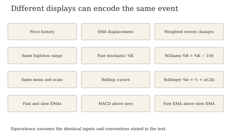
Figure 2. exact recodings under matched definitions. Other related indicators may share inputs without being identical.
Incremental value and the ablation question
Suppose a system already uses a 200-day trend filter and adds RSI, MACD, and three moving averages. The relevant experiment is not whether the combined system has a profitable history. It is whether each addition improves a declared outcome relative to the system without that addition, after including the extra search, trades, and fragility it introduces.
An ablation removes one component while preserving the rest of the protocol. If the removal changes turnover, risk, or decision frequency, report those changes. If a parameter was retuned after removing the component, this is a comparison of newly fitted systems, not a pure component test. Neither design is inherently wrong, but their interpretations differ.
A tool can also be redundant informationally and useful operationally. A dashboard may display both a raw spread and a standardized spread because the raw number answers a dollar question and the standardized number answers a scale question. The error is to multiply confidence as if two displays supplied two independent experiments.
Usefulness verdict
The universal dismissal of indicators fails: compression, risk measurement, execution, and finite-sample estimation can be useful. The universal promise of indicators also fails: formulas alone do not establish a favorable market distribution, affordable implementation, or superiority to a baseline. The rest of the book applies this four-part examination to particular families.
The mathematical demonstrations here are the author's finite-horizon arguments. The statistical chapter supplies research references for information, inference, and model selection; the distinction between actual and risk-neutral probabilities returns in the options chapter.
Why useful indicators may fail to produce a durable trading edge
An indicator can make a decision clearer without making its expected profit positive. ATR can express position size in units of recent volatility. A moving average can define when a system changes exposure. An oscillator can locate the present price within a chosen reference range. These are measurement and control functions. None supplies, by definition, the conditional distribution of the next tradable move or the cost of capturing it.
Empirical anchor. Bajgrowicz and Scaillet (2012), Technical trading revisited: False discoveries, persistence tests, and transaction costs, Journal of Financial Economics 106(3), 473–491, study 7,846 rules on daily DJIA prices from January 1897 to July 2011. Their persistence tests do not support selecting future superior rules in advance; low transaction costs eliminate the apparent in-sample performance they examine. They explicitly limit the implications for other markets and trading frequencies. Author manuscript, abstract and introduction.
The appropriate conclusion is that an indicator's usefulness does not establish a durable, executable trading edge. It would overstate this evidence to conclude that every indicator strategy must lose money, that every market is equally efficient, or that no intraday strategy can succeed. A single broad study is also insufficient to quantify what “most evidence” concludes across all instruments and methods.
Four reasons the inference fails
- Description does not determine prediction. A measured uptrend records how the chosen prices have behaved. To justify a profitable long trade, the decision maker still needs a favorable distribution of subsequent gains and losses at executable prices. A clear description is a necessary ingredient of a reproducible rule, not a sufficient condition for profit.
- The best historical setting is selected with hindsight. If many lookbacks, thresholds, exits, instruments, and date ranges are examined, the winner benefits from being chosen after its outcomes are known. The real decision is which rule to use before the next outcomes arrive. That requires a selection procedure evaluated on information it did not use, not merely a chart of the winning candidate.
- Small gross advantages can be consumed by turnover. Every change of position can incur spread, fees, slippage, and sometimes financing or borrowing costs. A signal that contains some predictive information may have no economic value for a trader whose execution costs exceed that information's payoff. Household evidence makes the same arithmetic concrete. Barber and Odean's study of 66,465 discount-brokerage accounts from 1991 to 1996 found that the most active traders earned 11.4% a year against a 17.9% market return; the average household earned 16.4% while turning over about 75% of its portfolio. After costs, trading was a performance penalty. The paper does not identify a particular indicator as the cause. It shows that activity itself can be the cost. Author paper.
- A relationship need not persist. A fitted association can depend on a particular volatility environment, liquidity condition, participant population, or research convention. More years of operation do not themselves force an unstable relationship to become favorable. Stability must be investigated rather than supplied by the word long-term.
These are analytical failure mechanisms, not a claim that this paper separately identifies the cause of every losing system. They explain why measurement, statistical predictability, implementability, and persistence are distinct requirements.
The expectancy arithmetic
For a specified strategy and opportunity population, let G be gross dollar profit and K be all trading costs. Assuming both expectations exist:
E[net profit] = E[G] − E[K].
Consider an invented example: a signal wins 55% of its trades, with a $100 average gross gain and a $100 average gross loss. Gross expectancy is 0.55 × $100 − 0.45 × $100 = $10 per trade. If average total costs are $15, net expectancy is −$5. Accurate predictions and negative net expectancy coexist without contradiction.
Under an unchanged distribution, repeating this example 1,000 times gives expected total net profit of −$5,000 by linearity. Independence is not required for that expectation, although dependence matters greatly for the distribution of losses and drawdowns. Trading longer does not repair a negative expected contribution. Conversely, this arithmetic does not establish that any actual indicator has those invented payoffs.
Positive return is not the same as an indicator edge
A strategy can have positive expected profit because it holds an asset with a positive expected return, while its indicator contributes nothing beyond a simpler exposure policy. It may even remain profitable while underperforming that policy after costs. Therefore “no demonstrated timing advantage,” “no statistically established excess return,” and “negative absolute expected profit” are different findings.
An indicator can also reduce exposure or help someone follow a plan while lowering both return and risk. That may improve the person's chosen objective. It does not prove a new source of expected profit. Specify whether usefulness means higher net return, lower risk, easier implementation, or more consistent behavior, and test that objective against a suitable comparison.
How to use an indicator honestly
Use it to define a measurable decision, then freeze the complete rule: market, information timing, entry, exit, sizing, and costs. Compare it with cash and a relevant simple exposure policy. Retain unfavorable variants, evaluate the selection procedure on genuinely unused observations, and report uncertainty and sensitivity to plausible costs. Claim an edge only to the extent that this evidence supports it.
The closing ORB study illustrates the distinction. An attractive published result warrants careful replication; our limited futures pilot neither reproduces that stock portfolio nor establishes a general theorem against breakouts. The same standard applies to favorable and unfavorable findings: preserve their actual scope.
Chapter 8
Data and Clocks
Most spectacular backtests begin with a small mistake about time. A daily high is treated as if it were known at the opening. A financial statement is assigned to its fiscal period rather than its publication date. A model learns from a database whose historical entries have been revised. A chart draws a pivot on Monday using prices that arrive on Thursday, and the trader remembers the mark as if it had been visible on Monday.
The geometric question is simple: which observations belong to Hₜ, the information set at the instant the order is chosen? The operational answer is rarely a single timestamp.
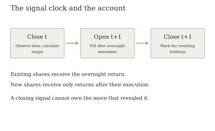
Figure 3. information and ownership change at different times. Execution must follow the observations used by the signal.
Four times for one observation
An event has an economic time, when the thing measured occurred. It has a release time, when an authorized source published it. It has an arrival time, when the trader's system received it. It has a usable time, when validation, calculation, and order construction were complete. A daily strategy may tolerate seconds of latency; a queue-position strategy may not. The same source can be adequate for one and unusable for the other.
A backtest must also distinguish an observation's original vintage from its latest corrected value. Revised macroeconomic data answer what statisticians now estimate happened. Point-in-time data answer what a trader could have known then. Both can support research, but only the second directly reconstructs the historical decision.
Proposition D1A daily bar does not determine the order of its intraday high and low.
Construction. Consider an open of 100, high 110, low 90, and close 105. One admissible path is 100→110→90→105. Another is 100→90→110→105. Both have the same OHLC bar. A long trade with a stop at 95 and profit target 108 reaches the target first on the first path and the stop first on the second. Its realized exit cannot be recovered from that bar alone. ∎
Corollary. A backtest that credits whichever order is favorable has introduced information the data do not contain. One can use finer data, specify conservative handling, or report a bound. Choosing the optimistic sequence without disclosure is not a fill model.
The same issue affects trailing stops and breakout entries. A bar can cross an entry level and a stop level without revealing whether the position existed when the stop was touched. Limit-order execution introduces an additional uncertainty: touching a price does not prove sufficient opposite-side liquidity reached the trader's place in the queue.
Proposition D2A symmetric pivot requiring future observations cannot be confirmed at the pivot time.
Definition. For k≥1, a k-sided pivot high at t satisfies Pₜ ≥ Pⱼ for every j from t−k through t+k, with a declared tie convention.
Demonstration. For a candidate already at least as high as the previous k observations, at time t values Pₜ₊₁ through Pₜ₊ₖ have not arrived. Construct two histories identical through t, one with all those future values below Pₜ and one with Pₜ₊₁ above Pₜ. The pivot classification differs although the available information is identical. It therefore cannot be determined from Hₜ. At the earliest, this definition can be evaluated when the last required future observation arrives. ∎
A chart is allowed to display the confirmed pivot at its economic location. A trading test must place the decision at the confirmation time. The distinction is especially important for ZigZag, fractal swings, centered filters, and pattern software that redraws an unfinished formation.
Prices, dividends, splits, and identity
A raw closing price is not a total return. A split changes quoted shares and prices without itself creating investor wealth. A cash dividend transfers value from the company to the holder and affects an ex-dividend price. Continuous futures series may splice contracts using offsets or ratios; the resulting chart need not be the historical price of any traded contract.
The laboratory uses a vendor-adjusted equity series and applies the same-date adjustment ratio to the open, high, and low. This is an explicit approximation to a consistent adjusted-price experiment. It is not a broker account ledger. The original study explains the remaining dividend and cash conventions, and does not separately add dividends already embedded in adjusted returns.
Proposition D3Mixing adjusted closes with unadjusted execution prices can create a fictitious return.
Construction. Consider two sessions before a later two-for-one split. The raw close and following raw open are both 100, so the economic overnight return is zero. A historical split-adjusted dataset reports the prior close as 50 and the following adjusted open as 50. Dividing the raw execution price 100 by the adjusted prior close 50 creates a fictitious 100% return. Dividing adjusted 50 by adjusted 50, or raw 100 by raw 100 over this pre-split interval, gives zero. The mixed convention is the error. ∎ by construction.
Scholium. A consistent adjustment does not repair every data problem. It does not create a point-in-time universe, correct a wrong timestamp, supply missing bid–ask spreads, or prove that a final-vintage adjustment was operationally available to a historical trader. Signal properties under rescaling should also be checked: some thresholds are invariant to multiplying all prices by a constant; dollar thresholds are not.
A universe is a historical object
Testing today's index constituents over earlier decades answers a question about survivors, not about the index that could have been held then. Deleted companies, mergers, bankruptcies, halted securities, exchange changes, and unavailable borrow are part of the opportunity set. A strategy that shorts only securities that survived long enough to enter a clean database can be biased in a different direction from a long-only survivor portfolio.
Delisting treatment depends on the database product. A vendor may supply a separate delisting return, an integrated total-return field, or a missing-code convention. Blindly multiplying a delisting adjustment into a return that already includes it double-counts the event. The necessary procedure is to read the field definition and reconcile a known example, not to apply a remembered recipe to every dataset.
The SPY study does not suffer stock-selection survivorship in the same manner as a retrospectively selected stock universe, because it evaluates one explicitly chosen surviving ETF. It still has selection limitations: choosing a successful U.S. equity fund as the entire test market limits the generalization. Calling a fixed-instrument study survivor-free without qualification would erase that distinction.
The data audit before the strategy audit
Record the provider, retrieval date, time zone, session definition, corporate-action treatment, missing values, duplicate records, instrument changes, and hashes of the actual input bytes. Reconcile several known events by hand. Inspect zero volume, repeated prices, implausible jumps, and changes in reporting conventions. A bar that looks unusual may be correct; an automated cleaning rule can remove genuine crashes precisely because they offend the model.
For an intraday strategy, specify whether timestamps mark the beginning or end of a bar, whether auctions are included, and how daylight-saving and overnight sessions are handled. For a multi-market strategy, distinguish a synchronized economic decision from a table whose rows share a calendar date but contain closes from different hours.
Usefulness verdict. OHLCV bars are useful summaries of a market. They do not contain a complete execution history. A visually plausible historical chart is necessary evidence for many strategies and sufficient evidence for very few. The burden of proof begins with the clock, before the first indicator is calculated.
Chapter 9
Moving Averages, Filters, and MACD
A moving average is a choice about memory. It exchanges some sensitivity to the latest observation for a summary of earlier ones. Its lag is not a software defect waiting to be removed by the right color scheme. It follows from assigning weight to the past.
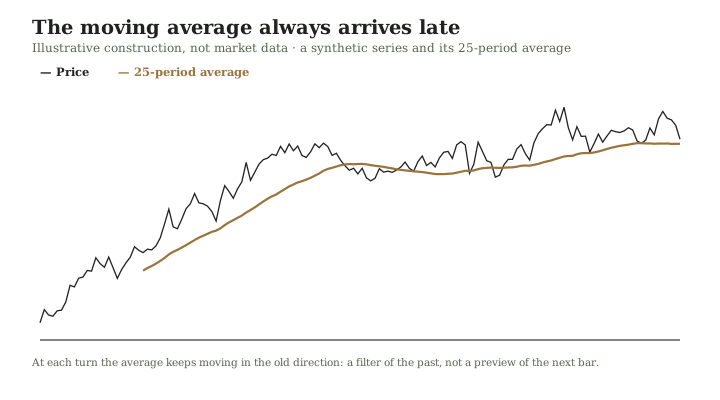
Figure 4. an illustrative construction, not market data. The average is a weighted memory of past prices; it cannot anticipate a turn it has not yet observed.
Let Pₜ be a consistently defined closing price. The n-observation simple moving average is Sₜ = (1/n)Σⱼ₌₀ⁿ⁻¹Pₜ₋ⱼ. An exponential moving average is Eₜ = αPₜ+(1−α)Eₜ₋₁, where 0<α≤1 and its initial value is stated. The familiar span convention uses α=2/(n+1); Wilder smoothing uses α=1/n. A span is not the same thing as a finite window: an EMA retains decaying weight on older observations.
Proposition F1Price minus its simple moving average is a weighted sum of recent price changes.
Assumptions. n≥2 and ΔPₜ=Pₜ−Pₜ₋₁.
Demonstration. Write Pₜ−Sₜ=(1/n)Σⱼ₌₁ⁿ⁻¹(Pₜ−Pₜ₋ⱼ). Each difference is Σₖ₌₀ʲ⁻¹ΔPₜ₋ₖ. The newest change appears n−1 times, the next n−2 times, and the oldest once. Thus
Pₜ−Sₜ = (1/n)Σₖ₌₀ⁿ⁻²(n−1−k)ΔPₜ₋ₖ.
∎
Consequence. “Price above the average” and “weighted recent momentum positive” are two descriptions of the same event under these conventions. They are not two independent witnesses. The identity concerns price changes, not percentage returns; substituting returns changes the exact weights and scale.
Proposition F2A causal weighted average has a calculable lag on a linear price path.
Assumptions. Mₜ=ΣⱼwⱼPₜ₋ⱼ with nonnegative weights summing to one and finite weighted age Σⱼjwⱼ. The path is Pₜ=a+bt over the observations used.
Demonstration. Substitute Pₜ₋ⱼ=Pₜ−bj. Then Mₜ=PₜΣⱼwⱼ−bΣⱼjwⱼ=Pₜ−bΣⱼjwⱼ. The price difference is slope b multiplied by weighted average age. For an n-point SMA, the age is(n−1)/2. ∎
For an EMA after the initialization term becomes negligible, weights are α(1−α)ʲ and their mean age is(1−α)/α. With the span convention α=2/(n+1), this is(n−1)/2, matching the SMA's mean age on a linear path. Their responses to reversals and noise still differ because equal mean age does not make their whole weighting distributions equal.
Worked case. On a path rising one dollar per session, a 20-day SMA trails the current price by 9.5 dollars. That difference is completely explained by the path and window. It is not a valuation discount and does not imply that price must return to the average.
Proposition F3Averaging independent measurement noise reduces its variance; the conclusion needs the independence premise.
Assumptions. Observations are a fixed level μ plus independent zero-mean errors εⱼ, each with varianceσ². A weighted estimate uses weights wⱼ summing to one.
Demonstration. Its noise is Σwⱼεⱼ. Independence removes covariance terms, giving varianceσ²Σwⱼ². Equal weights over n observations giveσ²/n. ∎
Boundary. A price is not generally a fixed signal plus independent measurement error. A random-walk level carries accumulated shocks, and averaging it changes exposure to those shocks rather than merely removing independent bad measurements. With correlated errors, the variance includes 2Σᵢ<ⱼwᵢwⱼCov(εᵢ,εⱼ). The popular claim that a moving average “removes noise” therefore requires a definition of noise and a model, not just a smoother-looking line.
MACD as a difference of memories
Under this edition's convention, MACDₜ=EMA₁₂(P)ₜ−EMA₂₆(P)ₜ. The signal line is EMA₉(MACD), and the histogram is MACD minus that signal line. An initialization convention matters near the beginning of a sample; the laboratory uses first-observation seeds and a long warm-up.
The MACD zero crossing compares two smoothed levels. A histogram zero crossing compares MACD with its own smoother. These are different decisions. A histogram can turn positive while MACD remains below zero; it says that the difference between two memories has improved relative to another memory, not that a universal bullish state has arrived.
Proposition F4MACD rejects a constant price level after the initialization transient.
Assumptions. Price is constant c, and both EMAs are initialized at c, or the limiting state is considered.
Demonstration. The EMA recursion preserves c because αc+(1−α)c=c. The difference of the two EMAs is therefore c−c=0. More generally, each EMA's deviation from c decays geometrically from its seed, so their difference tends to zero. ∎
This is a useful filter property. It does not mean that MACD extracts an independently existing force called momentum. It is a linear transformation with a particular response to temporal changes. On a rising ramp, the faster EMA lags less than the slower one, creating a positive difference. On a sufficiently persistent declining ramp, the sign reverses.
Crossovers and the price of responsiveness
A faster filter responds earlier to a reversal but also changes state more often in alternating prices. A slower filter suppresses some reversals and delays others. Neither dominates across all possible price paths. A smooth trend favors one tradeoff; a bounded alternating path favors another. A tuning exercise selects a compromise for the paths it has seen.
Consider closes 100,102,100,102,100,102. A very short threshold can repeatedly buy after an upward movement and sell after a downward movement. A long-window system may remain mostly unchanged. Now consider a permanent break from 100 to 70 followed by continued decline. The short rule may leave sooner. These constructions establish the absence of pathwise universal superiority, not the empirical frequency of either environment.
DEMA and TEMA combine exponential averages with negative coefficients to compensate for lag. A “zero-lag” formulation can have less lag on a chosen class of inputs by allowing overshoot or greater high-frequency sensitivity. The phrase must be read against the formula. No causal filter can know an arbitrary future reversal before the observations distinguishing that reversal arrive.
Percentage scaling and comparability
The percentage price oscillator divides a fast–slow difference by a price-level reference, making comparisons less dependent on the nominal price scale. Multiplying an entire price history by a positive constant multiplies ordinary MACD by that constant; a ratio oscillator can remain unchanged. Neither convention fixes all cross-asset comparability problems. Different volatilities, trading hours, price floors, and return distributions remain.
A dollar MACD threshold copied from a 20-dollar stock to a 2,000-dollar instrument has changed its economic meaning. A percentage threshold copied between an equity ETF and a volatile derivative can also imply very different risk. Standardization answers a scale question, not the entire portfolio question.
Usefulness verdict
Moving averages and MACD are useful, transparent ways to encode temporal weighting and form consistent state rules. Their algebra can be proved. Their future profitability cannot be inferred from that algebra. Use the raw-input comparison, a simple baseline, turnover, and an adverse-regime test before adding a second or third smoother. The added laboratory evaluates named fixed variants; it does not turn the winner of a finite table into the correct memory length for every market.
Source note. Indicator naming and historical attribution are documented in the historical chapter and technical-source register. Park and Irwin's survey of 95 modern technical-analysis studies found 56 positive, 20 negative, and 19 mixed results, with earlier profits more common in foreign exchange and futures than in equities, and with snooping and cost uncertainty still common enough that the positive count is not conclusive. F1–F4 are original derivations in this edition using the conventions stated above. Park and Irwin.
Chapter 10
Channels, Breakouts, and the Trend State
A breakout strategy buys a price that recently would have looked expensive. Its wager is not that expensive things are good. It is that a sufficiently strong movement can contain information about continued adjustment, and that occasional sustained moves can compensate for failed entries and trading costs. That economic hypothesis needs evidence. The channel merely makes the event measurable.
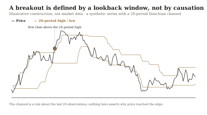
Figure 5. an illustrative construction, not market data. The channel is a rule about the last twenty observations; it asserts nothing about why price reached the edge.
For a prior-bars high channel define Uₜ=max(Hₜ₋₁,…,Hₜ₋ₙ). Define the low channel Lₜ=min(Lowₜ₋₁,…,Lowₜ₋ₘ). A closing-breakout example enters long when Cₜ>Uₜ, leaves when Cₜ<Lₜ, and retains its state otherwise. The order is scheduled for the following session. Entry and exit windows can differ. A rule that reverses short is a different strategy from one that holds cash; borrow, collateral, and upward equity drift make the distinction material.
Proposition T1A close cannot strictly exceed a high channel that includes its own bar.
Assumptions. A valid OHLC bar has Cₜ≤Hₜ, and a displayed upper channel is U*ₜ=max(Hₜ,…,Hₜ₋ₙ₊₁).
Demonstration. Cₜ≤Hₜ≤Uₜ, so Cₜ>Uₜ is impossible. ∎
Consequence. A plotted channel may legitimately include the present high. A strict close-breakout rule needs a reference that does not swallow the observation it is intended to test. Comparing today's close with yesterday's completed channel is one explicit convention. Comparing the intraday price with a resting stop-entry level is another, requiring a different fill simulation.
Proposition T2A fixed percentage filter is path-dependent, not just a fixed-horizon return threshold.
Construction. Start at 100 and consider a 10% trailing reversal from the highest price reached while long. Path A is 100→120→107. Path B is 100→105→107. Both end at 107 and have the same initial-to-final return. A has declined more than 10% from its high 120 and triggers the reversal; B has not. The return between the endpoints does not determine the filter state. ∎
This distinguishes the early percentage-filter literature from a simple rate-of-change oscillator. A filter carries an evolving extreme and a state transition. Historical attribution should not flatten these different systems into the claim that all trend followers use one formula.
The complete state machine
A strategy specification must say what happens before its first entry, during a signal tie, after an exit, and when both a risk override and a signal are present. “Buy breakouts” is not enough. An unambiguous long/cash machine has two states, with a separate execution queue:
- In cash, a confirmed upper-channel event schedules a long target for the next eligible fill.
- While long, a confirmed lower-channel event schedules cash.
- A missing input creates a declared response, such as retaining the last valid state while refusing new exposure.
- An operational stop overrides the signal only under its written rule; it is recorded as a separate decision.
The distinction between signal state and filled position prevents a common mistake. A long signal at the closing bell does not mean the account owned the preceding day's gain. An order can be pending, partially filled, rejected, or canceled. The backtest's ideal state transition is an implementation assumption, not a fact of market plumbing.
Proposition T3A trailing stop bounds a reference distance, not every realized loss.
Construction. A long position has a stop trigger at 95 after entry at 100. The next executable market opens at 80 with no eligible trades between. A sell stop that becomes a market order can fill near 80 rather than 95. Its loss exceeds the five-dollar trigger distance. A stop-limit order with a 95 limit can instead remain unfilled. Neither order supplies the universal five-dollar loss bound. ∎
Scholium. Stops can still be useful. They can make an exit rule consistent, reduce exposure to certain continuations, and control ordinary losses under specified liquidity conditions. Their usefulness is conditional; pretending they are insurance obscures exactly the rare event for which insurance would matter.
Why whipsaw is not an explanation by itself
A failed breakout is often called a whipsaw as if naming it explains why the system should survive it. The relevant quantities are the number, depth, timing, and correlation of such losses; the size and frequency of compensating gains; and whether the account can finance the waiting period. A system that earns most of its gains in a few sustained moves must stay implementable long enough to encounter them. That statement is not a promise that they will arrive.
A hypothetical sequence of ten losses of 1 followed by a gain of 15 has a positive gross sum. Change the gain to 8, or add costs of 0.6 to every trade, and the conclusion changes. The phrase “cut losses and let profits run” does not supply the missing distribution. The geometric foundation's expectancy and compounding results still govern the attractive story.
Multiple horizons and robustness
Combining several lookbacks can reduce dependence on a single parameter choice. It can also create correlated versions of the same exposure. A three-speed ensemble is not automatically three independent strategies. Evaluate how often the members disagree, how much their returns co-move, and whether the extra turnover earns its keep. A flat region of acceptable parameters is often more reassuring than one narrow historical peak, but even a plateau can be a property of a single market regime.
For a futures portfolio, normalize risk across contracts, specify rolls and financing, and account for the fact that contract multiplier and margin are different objects. The unlevered SPY laboratory below is deliberately narrower. Its 55/20 channel is a close-confirmed long/cash construction, not a replication of every Donchian or Turtle implementation. The Turtle chapter states Faith's published unit book and the modern public evidence that can, and cannot, be attached to it.
Evidence and verdict
Early filter investigations, the Brock–Lakonishok–LeBaron study, and the later Sullivan–Timmermann–White and Bajgrowicz–Scaillet studies answer different historical questions. The historical chapter records their scope. Diversified futures time-series momentum has its own evidence and should not be treated as the same experiment as a daily index breakout.
Channels are useful for defining extrema, states, and repeatable entries. They do not prove persistence, bound gap losses, or settle an optimal lookback. A defensible rule states which false starts it can afford and how its results compare with a simpler exposure policy.
Sources. Sullivan, Timmermann and White, author paper; Bajgrowicz and Scaillet. T1–T3 are this edition's original demonstrations.
Opening-range research
The special study at the end of this book contains the five-minute ORB research, opening RVOL formula, six geometric demonstrations, futures protocol, and preliminary backtest chart with long/short comparisons.
Chapter 11
RSI, Stochastic, CCI, and the Meaning of Strength
An oscillator places a recent movement on a scale. The scale can be bounded, centered, standardized, or smoothed. None of those choices supplies a natural law requiring the price to reverse at a marked line. The labels overbought and oversold are especially dangerous when they allow a description of a statistic to become a judgment about fair value.
Wilder's RSI
Let uₜ=max(Cₜ−Cₜ₋₁,0) and dₜ=max(Cₜ₋₁−Cₜ,0). Seed U and D with arithmetic averages of the first n changes, then update each using Wilder's recurrence: Uₜ=((n−1)Uₜ₋₁+uₜ)/n, and similarly for D. Define RSIₜ=100Uₜ/(Uₜ+Dₜ). If both terms vanish, this edition reports 50. If only D vanishes, RSI is 100; if only U vanishes, it is 0.
RSI measures strength relative to the instrument's own recent gains and losses. It is not the same as cross-sectional relative strength, which ranks one instrument against others. The two ideas share a phrase and answer different questions.
Proposition O1A high RSI does not entail a subsequent decline.
Construction. Let closing prices increase by one unit every session. After initialization, every dₜ is zero and every uₜ is one, giving RSI100. Continue the same path for any chosen finite number of sessions. There is no decline during that continuation. Thus the universal implication “RSI above 70 must soon reverse” is false for any fixed interpretation of soon. ∎
The counterexample also defeats the mirror assertion about a low RSI. It does not refute the empirical hypothesis that particular oversold events have attractive conditional returns in a stated market. A probabilistic reversal strategy must survive prolonged continuation; a continuation strategy must survive the reversal the oscillator did not guarantee.
Proposition O2Wilder smoothing and a conventional EMA can have the same update coefficient.
Assumptions. Wilder period is n; the conventional EMA uses span m and α=2/(m+1). Input and initial state are identical.
Demonstration. Equating 1/n with 2/(m+1) yields m=2n−1. Both recurrences then have identical coefficients. Equality of the initial state implies equality of all subsequent values by induction. ∎
Wilder 14 and EMA27 therefore have the same update coefficient, not Wilder 14 and EMA14. Different seeds still create different early values. RSI applies the smoothing separately to positive and negative changes before taking a ratio, so substituting an EMA of the RSI series is not the same transformation.
A worked RSI calculation
Take changes+2,−1,+3 and n=3. The initial smoothed gain is 5/3 and loss 1/3, so RSI=100×5/6≈83.33. Add a change−2. The next gain is 10/9 and loss 8/9, giving RSI≈55.56. This small example shows why the oscillator can fall substantially even though its smoothed gains remain positive: the ratio changes as recent losses enter the memory.
A14-period RSI and a 2-period RSI can represent very different trading behavior. A two-period reversal rule may enter frequently and hold briefly; costs and open-to-close timing can dominate its apparent edge. The laboratory reports both fixed variants, including all adverse comparisons, rather than choosing whichever threshold looked most persuasive after inspection.
Stochastic and Williams %R
For n completed bars, let Hⁿₜ be the highest high and Lⁿₜ the lowest low. The fast stochastic is %K=100(Cₜ−Lⁿₜ)/(Hⁿₜ−Lⁿₜ). A smoothing of %K is often called %D; platforms distinguish fast, slow, and full versions. Their smoothing choices must be specified. For a flat range, this edition assigns 50 rather than dividing by zero.
Williams %R under the conventional negative scale is−100(Hⁿₜ−Cₜ)/(Hⁿₜ−Lⁿₜ). The range can include the current bar because this statistic measures the close's location inside the range, not a strict breakout above that same range.
Proposition O3Fast stochastic and Williams %R are affine equivalents when they use the same range.
Assumptions. Hⁿₜ>Lⁿₜ, identical lookback and observations, no extra smoothing.
Demonstration. Subtract 100 from %K:100[(C−L)−(H−L)]/(H−L)=−100(H−C)/(H−L)=%R. Thus %R=%K−100. ∎
If %K is 80, %R is−20. A screen showing both values has shown the same location twice. Smoothing one but not the other changes the exact equivalence, yet it still does not justify an independence assumption.
CCI, rate of change, and scaling
A common Commodity Channel Index uses typical price T=(H+L+C)/3, its n-period mean M, and mean absolute deviation A=(1/n)Σ|Tⱼ−M|. Then CCI=(T−M)/(0.015A). The scaling constant is a convention. Mean absolute deviation is not standard deviation; silently substituting one changes the statistic. CCI is not confined to±100, and those conventional levels do not define a universal probability interval. For the fixed same-window formula above, it does have the finite bound derived below.
Rate of change over n periods is Cₜ/Cₜ₋ₙ−1 for positive denominators. An unscaled momentum indicator may instead report Cₜ−Cₜ₋ₙ. A percentage and a dollar difference can share a sign while disagreeing about cross-asset magnitude. Stochastic RSI applies a range-position calculation to RSI itself. It is an additional normalization of a derived series, not a new independently measured market variable.
Proposition O4The specified same-window CCI has a finite bound.
Assumptions. The window has n≥2 observations, includes the current typical price, and has positive mean absolute deviation A. Let d=T−M be the current residual.
Demonstration. All residuals sum to zero, so the other n−1 residuals sum to−d. Their absolute values sum to at least|d| by the triangle inequality. Including the current residual gives Σ|Tⱼ−M|≥2|d|. Thus A≥2|d|/n and |CCI|=|d|/(0.015A)≤n/0.03. ∎
For n=20 the bound is approximately 666.67. A window of nineteen zeros and one nonzero positive observation attains it. Thus the common informal description “unbounded oscillator” means that CCI is not restricted to the familiar±100 reference lines; it is not literally correct for this fixed-window definition. A definition using a different center or scale window needs a new analysis. If A=0, the ratio is undefined and the implementation must choose a neutral or missing value.
Divergence as an algorithmic question
“Price made a higher high while RSI made a lower high” sounds precise until the highs must be selected. Are they consecutive local extrema, the highest values in fixed windows, or manually chosen points? How many intervening bars are allowed? Is the oscillator high measured on the price-high date or at its own nearby peak? When is the second peak confirmed? What happens if it extends tomorrow?
A divergence hypothesis becomes testable only after those choices are made. The pivot proposition in Data and Clocks explains why a symmetrical peak label is unavailable at the moment it is plotted. A signal may correctly describe slowing recent momentum without predicting negative next returns. A car that decelerates can continue moving forward.
Usefulness verdict
Oscillators are useful normalizations and compact descriptions of recent behavior. RSI's ratio, stochastic's location, and CCI's deviation are different measurements, but none carries a built-in reversal mandate. Their usefulness depends on a complete continuation or reversal rule, execution timing, costs, and a regime comparison. A label such as oversold should never substitute for the expected-payoff calculation.
Sources. Fidelity's RSI definition, platform indicator reference, and Wilder's retrospective interview. These sources establish conventions and attribution, not profitable thresholds. O1–O3 are original demonstrations here.
Chapter 12
Bands, Ranges, and Volatility
A band answers where an observation lies relative to a chosen center and scale. A trader often asks it a different question: where must the next observation go? That substitution turns a descriptive interval into a prediction interval without doing the work needed to justify the change.
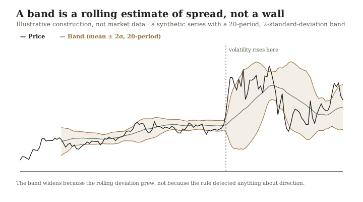
Figure 6. an illustrative construction, not market data. The band widens because the rolling deviation grew, not because the rule detected anything about direction.
For closes over n periods, let m be the arithmetic mean and s the population-standard-deviation convention, s²=(1/n)Σ(Cⱼ−m)². Bollinger-style bands are U=m+ks and L=m−ks. This edition uses the familiar 20-period, k=2 example when it names that rule. A sample-standard-deviation denominator n−1 gives different numerical bands. The platform convention belongs in the strategy specification.
Proposition B1Bollinger %b is an affine transformation of the rolling standardized deviation.
Assumptions. s>0 and k>0. Define z=(C−m)/s and %b=(C−L)/(U−L).
Demonstration. Substitute L=m−ks and U−L=2ks. Then %b=(C−m+ks)/(2ks)=1/2+z/(2k). ∎
For k=2, %b=1/2+z/4. A close at the upper band has z=2 and %b=1. Neither number is a probability. A screen that reports both has re-expressed one location, not collected an independent observation about the future.
Proposition B2Bands computed from past observations provide no distribution-free coverage guarantee for the next price.
Construction. Fix any finite observed history with finite band endpoints L and U. Continue it with next price U+M for some M>0, or with a positive price below L when such a price is permitted. The historical band is unchanged because its inputs are unchanged, yet the next observation falls outside it. A probability law can place any desired mass on such continuations unless further restrictions are imposed. Therefore no fixed future coverage percentage follows from the band formula alone. ∎
Even under independent normal observations with unknown mean and variance, a predictive interval for a new observation must account for estimation uncertainty and a new observation's variation. A band fit to rolling, dependent price levels is a different object again. The familiar normal-distribution statement about a known mean and standard deviation cannot simply be pasted onto it.
John Bollinger's own rules warn against treating a band touch as a complete buy or sell signal. A touch can be used in a reversal hypothesis, a continuation hypothesis, or a conditional risk rule. These are different policies with opposite trades, and the formula does not choose among them. Bollinger's rules.
Proposition B4An observation standardized by its own fixed window has a finite geometric limit.
Assumptions. The n≥2 observations include C, the mean is their arithmetic mean m, and population standard deviation s is positive. Let a=C−m.
Demonstration. The remaining residuals sum to−a. Cauchy–Schwarz gives their squared sum at least a²/(n−1). Thus ns²≥a²+a²/(n−1)=na²/(n−1), giving |(C−m)/s|≤√(n−1). ∎
With n=20, the current included observation cannot have |z| greater than√19≈4.36 under this exact convention. A future observation standardized using a previously fixed window has no such algebraic bound. This is another reason to distinguish fitted bands from forecasting intervals: they are different mathematical objects before any market data are examined.
A narrow band does not choose a direction
Bandwidth is often(U−L)/m, with percentage scaling stated explicitly. A squeeze says recent dispersion is small relative to the chosen center. It does not establish when dispersion will increase, how much it will increase, or whether the next large move will be upward. Comparing Bollinger and Keltner widths combines two dispersion estimates; it does not create a direction forecast by algebra.
A low-volatility period can precede a large move because volatility changes. It can also remain quiet for a long time. An option buyer pays for the market's forecast of that possibility. The options chapter explains why correctly anticipating movement is not enough if the option's price already exceeds the value of the realized movement.
True range and ATR
True range is TRₜ=max(Hₜ−Lₜ,|Hₜ−Cₜ₋₁|,|Lₜ−Cₜ₋₁|). It includes gaps that a within-bar high-minus-low range can miss. ATR smooths true range, commonly with Wilder's coefficient 1/n and an explicit initial average. It has price units. ATR divided by price gives a relative scale when price is positive, but still is not a standard deviation unless a model connects them.
Proposition B3ATR alone cannot identify the direction of a reflected price path.
Construction. Apply the reflection C′=A−C with a sufficiently large constant A, so that C′=A−C, H′=A−L, and L′=A−H remain valid positive prices over the finite example. The within-bar range is unchanged, and the two gap magnitudes exchange roles. True range is unchanged on every bar, hence ATR is unchanged with the same seed. Upward changes have become downward changes. Direction therefore cannot be recovered from ATR alone. ∎
This is a structural reason to evaluate ATR as a range/risk measure rather than a signed predictor. ATR can enter a directional system together with other data, but the direction then comes from the joint rule, not from ATR's sign, which is nonnegative.
Risk units and their limits
If intended account risk is B dollars, entry price is P, ATR>0, k>0, and the planned stop lies k ATR below entry, a position size q=B/(k ATR) gives a modeled stop-distance loss B. Contract multipliers must be included when q denotes contracts. Commissions, spread, slippage, gaps, and discrete lot sizes alter the realized loss. A low ATR can increase the proposed quantity just before volatility expands; an exposure cap therefore serves a different purpose from range normalization.
Take B=500 dollars, ATR=2 dollars, and k=2. The formula gives 125 shares. A fill four dollars below entry loses 500 before costs. A gap eight dollars below entry loses 1,000 before costs. The arithmetic proves both statements. It cannot decide which future fill occurs.
Keltner-style channels use a center such as an EMA and an ATR multiple. Historical and platform variants differ; the exact chosen formula should be written. Replacing a standard-deviation band with an ATR band changes sensitivity to closes, intrabar ranges, and gaps. Neither convention is universally superior across all paths.
Volatility is an estimate of a distribution, not a maximum loss
Realized volatility commonly annualizes a daily return standard deviation by √252. That scaling is a convention motivated by particular temporal assumptions; it is not a law that a market has 252 independent opportunities for a normal shock. Serial dependence, volatility clustering, fat tails, and changing trading calendars affect interpretation. A10% volatility target is not a 10% maximum drawdown target.
A variance forecast can be evaluated with an appropriate forecast loss and then with the performance of the sizing policy it supports. Those two evaluations need not agree. An accurate forecast may arrive too late to reduce a gap loss, and an imperfect forecast may still stabilize exposure relative to a completely constant notional position.
Usefulness verdict
Bands and ranges are useful ways to normalize distance, compare states, and size positions under a declared model. A two-standard-deviation band does not prove 95% next-price coverage. A squeeze does not choose direction. ATR does not guarantee a stop fill. Their most defensible uses begin by respecting these limits, then asking whether the resulting rule improves a specified objective after costs.
Sources. Bollinger's construction; ATR formula and recurrence. B1–B3 and the risk arithmetic are this edition's demonstrations.
Chapter 13
Directional Movement and the Claim of Trend Strength
“Strong trend” can mean a large signed return, a smooth path, persistent positive autocorrelation, a high signal-to-noise ratio, or a particular indicator value. These meanings are not equivalent. A large overnight jump followed by inactivity can produce a large return without persistent directional trading opportunities. A steadily drifting path can be smooth and still too small to pay a spread.
Wilder's directional movement system offers one precise construction. Set up=Hₜ−Hₜ₋₁ and down=Lₜ₋₁−Lₜ. Positive directional movement is up when up>down and up>0, otherwise zero. Negative directional movement is down when down>up and down>0, otherwise zero. This edition assigns both zero on a tie. Smooth these series and true range consistently. Then +DI=100 smoothed(+DM)/ATR and −DI=100 smoothed(−DM)/ATR where denominators are positive. DX=100|+DI−(−DI)|/(+DI+−DI), with DX=0 when the sum is zero in this edition. ADX smooths DX.
Proposition W1ADX can be identical on opposite directional paths.
Assumptions. Reflect a finite valid OHLC path as in Proposition B3 and use matching smoothing/initialization conventions.
Demonstration. Reflection exchanges upward and downward movements, so +DM and −DM exchange roles. True range remains unchanged. Therefore +DI and −DI exchange roles. The absolute difference and sum in DX do not change, so DX and its smoothed ADX do not change. The direction of the underlying path has reversed. ∎
A high ADX does not, by itself, mean bullish. The sign or direction must come from another component, such as the ordering of +DI and −DI, price relative to a filter, or a separate return signal. This is not a criticism of ADX; it is the difference between the statistic's intended role and a misuse of it.
Proposition W2A fixed threshold on a smoothed statistic can remain satisfied after its unsmoothed input changes.
Assumptions. A statistic follows Aₜ=αXₜ+(1−α)Aₜ₋₁ with 0<α<1. At t−1, Aₜ₋₁ is above a positive threshold h. Subsequent input is zero.
Demonstration. Iteration gives Aₜ₋₁₊ₖ=(1−α)ᵏAₜ₋₁. It remains above h for every k satisfying(1−α)ᵏAₜ₋₁>h. Thus a threshold can persist while the current input supplies none of the earlier strength. ∎
Applied to an ADX-like smoother, this explains why a high value can be a memory of directional behavior rather than confirmation that the same behavior will continue. A falling ADX can coexist with continued price appreciation; the statistic is not a signed price change.
Gating a strategy creates a new strategy
Suppose a crossover system trades only when ADX exceeds 25. The gate changes which observations enter the payoff distribution, how long the account stays in cash, and how frequently transitions occur. It may remove costly alternating periods. It may also remove the early part of a profitable trend while waiting for the measure to rise. Both mechanisms are plausible. Their balance is empirical.
The fair comparison is the ungated system, the gated system, and a simpler exposure or turnover reduction chosen without using the final evaluation period. If the gated system has lower volatility because it is invested half as often, that is useful descriptive evidence but insufficient evidence of superior trend identification. Report conditional return, time invested, missed moves, and cost changes together.
A threshold selected after comparing 15,20,25,30,35 and several smoothing lengths belongs to a family of tried strategies. Presenting only 25 does not reduce the number of decisions that produced it. The inference chapter explains how a tidy final rule can hide an untidy search.
Parabolic SAR and the moving exit
A parabolic stop-and-reverse construction maintains an extreme point and an acceleration factor, moving a stop toward the favorable extreme as a trend progresses. Exact clamps against recent highs/lows, acceleration increments, maximum acceleration, reversal handling, and initialization vary by implementation. A formula copied without those state details is not a fully specified strategy.
A mechanically tightening exit can reduce the room available to a reversal. It can also force frequent exits from a trend whose ordinary fluctuations exceed that room. A stop-and-reverse version adds opposite exposure; a stop-only version does not. Neither inherits a guarantee from the word parabolic.
A practical diagnostic
Before using a strength gate, draw three synthetic paths: a steady ramp, a single jump followed by a flat level, and an alternating range. Compute the statistic using the exact platform settings. Observe its warm-up, its persistence, and its response to a sudden reversal. These exercises test whether you understand the object. They do not estimate its market profitability.
Then ask a specific empirical question. For example: does the gate improve the net return of an already specified trend rule relative to reducing its exposure by a constant fraction? A study of that question can be informative. A chart showing a high indicator value during a retrospectively selected trend cannot answer it.
Usefulness verdict
Directional movement systems provide reproducible distinctions between signed directional components and a smoothed strength statistic. They are useful for describing and conditioning a strategy. They do not establish direction from ADX alone, prove persistence, or make conventional thresholds optimal. Their value should be assessed as an addition to a complete policy, with the cost of late confirmation and missed opportunities included.
Sources. Wilder's own account of his 1978 systems; platform formulas and conventions. W1–W2 are original demonstrations in this edition.
Chapter 14
Volume, Breadth, VWAP, and the Auction
Every completed trade has a buyer and a seller. Volume is not net money entering a market. A price can rise on low volume, fall on high volume, or change because the marginal available quote changes while many holders do nothing. Volume becomes informative through a model of who trades, why, at what price, and with what constraints, not through the assertion that buyers have outnumbered sellers in completed transactions.
On-balance volume
Define OBVₜ=OBVₜ₋₁+Vₜ sign(Cₜ−Cₜ₋₁), assigning zero on an unchanged close and choosing an initial level. The whole bar's volume receives the sign of the bar's close-to-close change. That makes OBV a signed-volume construction, not an observation of buyer-initiated minus seller-initiated transactions.
Proposition V1OBV loses price-change magnitude and has an arbitrary additive origin.
Construction. A close moves from 100 to 100.01 on one million shares, or from 100 to 110 on the same volume. Both cases add one million to OBV. The OBV increment cannot distinguish the two return magnitudes. Further, replacing the initial OBV by OBV₀+c adds c to every subsequent value by induction, leaving changes unchanged. ∎
The loss of magnitude is a design choice, not proof of uselessness. It may separate participation from price scale. But a particular absolute OBV level has no invariant interpretation unless its initialization is fixed. A divergence needs an exact definition of the price and OBV extrema it compares.
Accumulation/distribution constructions weight volume by the close's location within the bar, often using[(C−L)−(H−C)]/(H−L). Chaikin-style money flow aggregates such weighted volume and normalizes by total volume. Money Flow Index uses changes in typical price to classify price-times-volume observations. These are distinct compressions of OHLCV. None is a direct census of informed investors' cash flows. Flat ranges and zero-volume denominators require declared handling.
Proposition V2Aggregated OHLCV cannot uniquely recover trade initiation or order-book history.
Construction. Two sequences of trades can have the same prices, sizes, open, high, low, close, and total volume while the prevailing bid and ask differ at each trade time. A trade at 100 may occur at the ask in one quote sequence and at the bid in another. The OHLCV summary is identical, but a quote-based initiation label differs. ∎
A bar-based approximation can still be studied. It must not be advertised as exact order flow. Genuine aggressor flags, consolidated quote matching, and venue-specific feeds have their own timestamp, coverage, and classification problems. They belong to a different data tier from a colored volume bar.
VWAP as an execution reference
For trades with prices pᵢ and positive quantities vᵢ over a declared interval, VWAP=Σpᵢvᵢ/Σvᵢ. Specify whether auctions, off-exchange reports, corrections, and particular venues are included. A bar-based approximation that multiplies a representative bar price by bar volume is not necessarily the trade-level statistic.
Proposition V3VWAP lies between the minimum and maximum included trade prices.
Assumptions. All vᵢ≥0 and total volume is positive.
Demonstration. Weights wᵢ=vᵢ/Σvᵢ are nonnegative and sum to one. Since p_min≤pᵢ≤p_max, multiplying by wᵢ and summing gives p_min≤Σwᵢpᵢ≤p_max. ∎
That is a valid mathematical property. It does not say that a price below VWAP is undervalued or must recover. VWAP is the average of included executed prices, not an equilibrium value. The full day's final VWAP is also unknown at the day's start; a real-time cumulative VWAP and an execution algorithm's forecast of final volume are different objects.
Anchoring chooses a history
The short statement is this: an anchored VWAP is a VWAP whose accumulation start is a chosen event rather than the session open. Everything that follows is the complete reference. The geometry, the platform formula, the institutional benchmark, the hindsight trap, and the absence of a livelihood study are different facts. They share a line on a screen.
The anchored VWAP
Three objects share the letters. Confusing them is how a useful average becomes a prophecy.
Trade-level VWAP. For included prints with prices pᵢ and positive sizes vᵢ, VWAP = (Σ pᵢ vᵢ) / (Σ vᵢ).
This is the object Berkowitz, Logue, and Noser introduced in 1988 as a naive-trader execution benchmark on the NYSE: the volume-weighted average of the day’s transactions, against which a desk’s fills can be compared. In their sample of more than 14,000 institutional trades, total costs averaged about 23 basis points of principal, of which about 5 were the impact component under that measure. The paper is about measurement of a completed order. It does not say that price must revert to the average. Journal of Finance
Bar VWAP. Platforms rarely have every print. They substitute a bar source, most often the typical price (H+L+C)/3, sometimes (H+L)/2, times the bar’s volume, then accumulate. TradingView’s official VWAP does exactly that, default source hlc3. Official calculation
Session VWAP versus anchored VWAP. Session VWAP resets when the declared session, week, month, earnings date, or other calendar/corporate clock restarts. Anchored VWAP (AVWAP) is the same running ratio begun at a user-chosen bar. Brian Shannon’s public definition is the clean one: it is VWAP “except the start point (the anchor) … is set by the user at a specific meaningful point.” AlphaTrends
Paul Levine’s MIDAS work (1995–1997), developing Kevin Haggerty’s 1980s use of VWAP curves, is the technical-analysis ancestor. TradingView’s drawing-tool note records that lineage and names Shannon, Zach Hurwitz, and the CMT Association as the popularizers. A lineage is not a test. Drawing tool
Proposition V4A typical-price bar VWAP need not equal the trade-level VWAP of the same interval.
Construction. A bar trades 90 at 100 shares, then 110 at 100 shares, then 100 at 800 shares. Trade-level VWAP is (90×100 + 110×100 + 100×800) / 1000 = 100. The bar’s high, low, and close are 110, 90, and 100, so typical price is 100 and the bar VWAP is 100 in this case. Change the last print to 104 at 800 shares: close is 104, typical price is (110+90+104)/3 = 101.333…, bar VWAP is 101.333…. Trade-level VWAP is (90×100 + 110×100 + 104×800) / 1000 = 102.4. The two averages disagree. ∎
The disagreement grows when volume clusters at one extreme of the bar, when the open is far from the typical price and is omitted from hlc3, or when the feed’s “volume” is tick count rather than shares. Shannon is right that tick data are the accurate institutional object and that a one-minute bar is a compromise. The compromise is a different statistic. Always state which one is on the screen.
The running-sum identity
Let S be the running sum of (source × volume) from the anchor through the current bar, and let V be the running sum of included volume. AVWAP = S / V whenever V is positive. The next print with source s and volume v updates the average to
AVWAP_new = AVWAP + [v / (V + v)] × (s − AVWAP).
Proposition V5A new print moves the anchored VWAP toward that print by the print’s share of cumulative volume.
Assumptions. Prior cumulative volume V is positive, the new volume v is nonnegative, and V + v is positive.
Demonstration. The displayed identity is algebra on the updated sum S + s v. The weight v / (V + v) is the new print’s share of all included volume. ∎
This is why a late, heavy bar yanks the line and a quiet bar barely moves it. It is also why “AVWAP is slow late in the day” is not a mystery: the denominator has grown. TradingView’s own help page says the same thing about session VWAP lag as the close approaches. Lag is the average doing its job. It is not a defect to be offset by dragging the line.
A platform offset that shifts the plotted line forward or backward is a display displacement. TradingView documents it as an input. Using a backward offset as if the average had been known earlier is the same error already forbidden for a detrended price oscillator. The number was calculated at the bar. The plot is not a time machine.
What the line is not
AVWAP is the average of the included source prices, weighted by the included volume definition, from the included start. It is not:
- the average entry of “the longs,”
- the average entry of “the shorts,”
- a census of open interest or remaining inventory,
- an equilibrium value,
- a promise that price below the line is cheap,
- a promise that institutions must defend it.
Every completed trade has two sides. Weighting by volume does not reveal who was urgent. Proposition V2 already forbids recovering initiation from OHLCV. Shannon’s public page is careful on one point and loose on another: he notes that volume is both buying and selling, then writes that AVWAP “shows us which side is in control.” Slope of an average of included prices is a description of that average. It is not a unique identification of an aggressive party.
Proposition V6Price below an anchored VWAP does not entail that included participants have a mark-to-market loss on their inventories.
Construction. From the anchor, 1,000 shares print at 100 and 1,000 at 110. AVWAP is 105. Price is now 104. A participant who bought the entire 100 print and sold the entire 110 print is flat and has a realized gain of 10 per share on that round trip. A participant who shorted 2,000 at 110 and is still short is marking a gain. A participant who bought 100 at 100 and still holds is marking a gain. None of these inventories can be read from the fact that 104 < 105. ∎
“Below AVWAP, the bulls are trapped” is a story about an inventory the chart does not contain. The honest sentence is: the last price is below the included average of the chosen source. V3 already places that average between the minimum and maximum included prices. It does not place anyone’s book.
Choosing an anchor is choosing a history
The economically motivated list is short and should be written before the mouse click.
| Class | Example | Clock that makes it eligible |
|---|---|---|
| Calendar | Session open, week, month, year, IPO day | The clock, known in advance |
| Corporate | Earnings release, dividend, split | The announced timestamp, not the subsequent drift |
| Macro | FOMC statement, scheduled data | The scheduled minute |
| Gap / range | First print after a defined overnight gap | The gap definition, fixed before the open |
| Confirmed swing | A low or high that has already satisfied a written confirmation rule | The confirmation bar, not the extremum itself |
| Discretionary | “This looks important” | Admit that the event is the click |
TradingView’s session VWAP can reset on Session, Week, Month, Quarter, Year, Decade, Century, Earnings, Dividends, or Splits. Those are platform clocks. They are still model choices. An earnings reset that uses the vendor’s earnings timestamp is a different experiment from a reset at the first regular-hours bar after the print.
Shannon’s public page contains the confession that most discretionary AVWAP charts omit. On a one-minute example he draws a second line from the day’s low and writes that it is drawn in “only after it is obvious that it was an important low.” That line is a description of a completed morning. It was not a decision rule at 11:01. The later touches that “held” are interesting as description. They are not a test of a rule that could have been run at the low.
Proposition V7An anchor chosen using subsequent prices is not available at the candidate event.
Assumptions. A candidate bar t₀ is eligible as an anchor only after a later condition on prices after t₀ becomes true. The decision at t₀ may use only information in H at t₀.
Demonstration. The later condition is not a function of H at t₀. Any policy that waits for that condition and then treats t₀ as if it had been the live anchor is using a later history. That is a different information set from the policy that must choose at t₀. ∎
The correct live objects are: (i) a clock-based anchor known at t₀ (the open, the release), or (ii) a confirmation-time anchor whose first plotted point is the confirmation bar, with the line accumulated from a predeclared rule that does not peek. Plotting from the unconfirmed low and scoring the bounce that defined the low is the retest error of C3 in volume-weighted clothing.
If several anchors are shown, write why each qualified and when. Moving an anchor after an unfavorable break is a new strategy. So is adding a third AVWAP because the first two failed to “hold.”
Bands are a second model
TradingView’s VWAP bands are, officially, standard deviations of the VWAP values since the last anchor, optionally scaled as a percent, then multiplied by a user factor. They are not Bollinger bands on price. They are not a statement that 95% of future prints will lie inside two standard deviations.
Proposition V8A standard-deviation band of the AVWAP series is not a standard-deviation band of the included prices.
Construction. Let included source prices be 90, 110, 90, 110, each with equal volume. AVWAP after four prints is 100, and the series of AVWAP values is 90, 100, 96.667, 100, tight. The standard deviation of the four prices is 10. A one-standard-deviation band around 100 built from the AVWAP series is much narrower than a one-standard-deviation band built from the prices. A print at 108 can lie outside the price band and inside the AVWAP-series band, or the reverse if the average has trended. ∎
A fade of “2σ AVWAP” is a fade of a platform object. State which σ. State that it is not a probability. State the fill.
Several lines are several histories
Two AVWAPs are two running-sum pairs. Their crossing is an event in the pair of averages. It is not a third observation, and it is not confirmation in the sense of independent evidence. Under U2, an invertible recoding of one line is the same line. A second anchor is a different function of H only because it drops a different prefix of the tape. That can be useful as a scenario: “since the gap” versus “since the open.” It cannot be multiplied into two experiments.
“Confluence” of three AVWAPs plus a session VWAP is four running means of overlapping subsets of the same prints. Treat it as a description of those subsets. Do not treat it as four voters.
Strategies as sold, and what they actually are
| Sold as | Actual object | What would make it a test |
|---|---|---|
| Institutions defend AVWAP | A hypothesis about other people’s inventory and urgency | Identified order flow, not the average itself |
| Rising AVWAP is support | A description that a rising average often lies below a rising price, partly by construction of an average | A predeclared touch-and-bounce rule, confirmation clock, costs, and a simpler trend alternative |
| Fade extended bands | A fade of a platform σ of the average path | The band definition, hold, stop, and a volatility-target control |
| Reclaim is a long | A cross of last price through a running mean | Next-open or next-trade fill, not the signal bar’s close |
| Year-to-date AVWAP is “the institution’s cost” | A calendar-reset bar average | The same problems as V6, plus January concentration and index rebalance flow |
| Beat VWAP, therefore good trade | An execution grade | E1: a fill below interval VWAP can still lose money on the asset |
Shannon’s CMT slides say trades should generally be in the direction of AVWAP and that a rising AVWAP “will often act as support.” Those are practitioner maxims. This edition does not reconstruct his book’s charts. The marketing sentence that the book will help the reader “make more money” is a sales claim. CMT slides
No inspected journal study freezes “buy the first confirmed reclaim of AVWAP from a predeclared event” or “fade two AVWAP-series σ” on a stated universe, with costs and a snooping control. The execution literature is large and is about desks. The chart literature is practitioner and promotional. That gap is the result of the search, not a missing compliment.
Session VWAP as a game, not a magnet
A desk graded on beating session VWAP has an incentive to trade with volume and to avoid looking different from the day’s average. Madhavan records how the benchmark changes placement, horizon, and venue. A guaranteed-VWAP product transfers the tracking problem to a broker. None of that implies that your next scalp should fade the line. It implies that some large orders are scheduled toward the line. Participation can lean on a known average without making that average a mean-reverting law. Madhavan 2002
A simulation that allocates an order using the realized future volume curve has given the algorithm the day’s tape. The execution chapter already forbids that as a hindsight schedule. The same prohibition applies to an AVWAP “reclaim” that uses the day’s final volume to decide whether the morning cross “counted.”
Where the number breaks
Volume definition. Shares, contracts, notional, or tick count. Crypto and some FX feeds offer ticks. Tick-AVWAP is not share-AVWAP.
Session filter. Premarket and postmarket can be in or out. Shannon notes the choice. A gap-anchor that includes the print and a session VWAP that excludes premarket are different histories of the same morning.
Corporate actions. A split changes the price series. A platform “Splits” reset is one convention; an unadjusted cumulative sum across the split is another. Dividends do not enter a price-only VWAP unless the source is total-return, which these tools are not.
Futures rolls. A continuous chart splices contracts. Volume on the back month does not belong in an AVWAP started on the front month unless the roll rule says so. State the contract.
Open, equality, zero volume. The first included bar with zero volume is undefined as a ratio. Platforms substitute the source price. Write the rule.
Higher-timeframe display. TradingView can compute VWAP on one timeframe and plot it on another, optionally waiting for the higher bar to close. A 5-minute chart showing an hourly AVWAP that updates before the hour closes is a different information clock from one that waits. U1 still applies: the line is a function of H. The question is which H.
A worksheet before the line is used as a trade
| Field | What to write |
|---|---|
| Object | Trade VWAP, bar VWAP (hlc3, hl2, close, …), or mixed |
| Volume | Shares, contracts, notional, ticks; which session |
| Anchor | Clock, release, or confirmation rule; the exact timestamp |
| First eligible decision | The first bar at which that anchor is known |
| Role | Execution benchmark, descriptive reference, or trade trigger |
| If a trigger | Entry, stop, exit, size; next-print fill |
| Comparison | The same rule with the AVWAP removed, and a simpler trend or cash alternative |
| Rejection | The observation that retires this anchor family |
If the role is execution, grade fills against the stated interval and keep investment P&L on a separate line (E1). If the role is description, do not speak of trapped bulls. If the role is a trigger, the laboratory’s next-open discipline applies: the state at the close of a bar is an instruction for a later print.
What this edition will not claim
AVWAP is one of the few popular tools whose institutional use is documented in a top journal as a benchmark. That is a real distinction from a stochastic oscillator. It does not make the retail reclaim a proven edge. It does not make Shannon’s subjectivity a virtue. It does not make three overlapping averages into independent evidence. The best use in this book is the honest one: a declared average of a declared history, useful for execution and for saying “since that event, the included average is here,” and silent about who must defend it.
Breadth requires the right denominator
Market breadth can count advancing versus declining instruments, new highs versus lows, or members above their own moving averages. Its interpretation depends on the universe and weighting. Fifty small advancing stocks and one very large declining stock can produce positive equal-weight breadth while a capitalization-weighted index falls. That is a difference in aggregation, not a contradiction.
A historical breadth series must use constituents and eligible securities known at the time. Today's surviving members create a different experiment. Listing counts, closed-end funds, multiple share classes, and exchange migrations can change the denominator. A breadth divergence should therefore be interpreted only after its membership definition is stable enough to support comparison.
Volume profiles and market profiles
A volume profile allocates traded quantity across price bins. A time-based market profile allocates observations or time-price opportunities across bins. Bin width, session boundaries, composite windows, and data coverage influence visible nodes. A high-volume node records where substantial trading occurred under those conventions. It does not prove that unfilled demand remains there or that the same participants will defend it later.
Profiles can support a consistent auction description and order-location hypothesis. Their predictive use requires an explicit event definition: for example, what counts as a return to a prior value area, when the area becomes fixed, and whether the entry is a market order or a limit that may not fill. The execution chapter explains why an attractive limit price and a completed profitable trade are separate events.
Evidence and verdict
Volume contains an input absent from close-only indicators, so it can add information relative to a close-only baseline. That possibility is not proof that a particular volume transform does so usefully. Test its incremental contribution using the same market, horizon, execution, and search accounting. Do not multiply confidence merely because several volume indicators share the same underlying Vₜ.
VWAP is especially useful as a defined benchmark and execution objective. Anchored VWAP is the same average with a chosen start: useful as a declared history, silent about trapped inventory, and untested here as a reclaim or fade livelihood. OBV, breadth, and profiles can be useful descriptive or predictive features. Their strongest common misuse is to turn an aggregate statistic into a story about hidden intent without evidence capable of identifying that intent.
Sources. Primary archival research on OBV's precursors and Granville's popularization; platform definitions; Berkowitz, Logue and Noser; TradingView VWAP; TradingView AVWAP; Shannon / AlphaTrends; Madhavan 2002. Inspected notes are in books/research/expansion/anchored-vwap-sources.md. The execution and microstructure chapters provide the research basis for benchmark and order-flow analysis. V1–V8 are original demonstrations here.
Chapter 15
Candles, Patterns, Support, and Resistance
A chart pattern is a hypothesis about the relationship between a shape and a subsequent outcome. It becomes research when another person can locate the same shape without seeing that outcome. The quality of the drawing is secondary to the independence of the labeling.
Candlesticks summarize the relationship among open, high, low, and close. A body is the open-to-close interval; wicks show the remaining high and low excursions. A hammer, engulfing formation, or doji adds rules about relative sizes and sometimes about preceding context. A label without a tolerance, context window, and confirmation rule is not yet a reproducible event.
Proposition C1The same candle can be followed by opposite returns.
Construction. Fix a completed bar with open 100, high 105, low 90, and close 104, and fix every preceding observation. Continue one price path with a rise to 110 and another with a fall to 95 at the next executable observation. Both histories contain the identical long-lower-wick candle; the subsequent return signs differ. Therefore the candle cannot logically entail a positive next return. ∎
This does not imply equal probabilities for those continuations. It establishes that a directional probability needs an empirical or structural premise. The same distinction applies to a bullish engulfing formation, an outside bar, and a sequence of candles described as accumulation.
From a picture to an event
A reproducible double-top hypothesis might specify two confirmed peaks separated by a minimum number of bars, a maximum percentage difference between peak heights, a minimum intervening decline, and a break below the intervening low. Every choice matters. Confirmed peaks arrive after their economic locations; the trade occurs only after confirmation and the declared break. A neckline drawn through the most convenient later points is not a pre-existing price level.
A head-and-shoulders detector additionally needs rules for the relative head height, shoulder symmetry, duration, neckline slope, and permitted noise. A triangle needs rules for choosing its boundary points and for ending the formation. A flag needs a definition of the preceding impulse, the consolidation, and the breakout. Increasing the flexibility of these descriptions increases the number of shapes that can be recognized after the fact.
The purpose of formalization is not to declare that a human eye has no value. It is to make clear which part of the process is being evaluated. Human labels can be studied with blinded examples and inter-rater agreement. An algorithm can be studied on a frozen event set. Both fail when the future is visible during labeling.
Proposition C2A distributional pattern effect need not imply a directional trading edge.
Construction. Without a pattern, let next return be equally likely+2% or−2%. Conditional on the pattern, let it be equally likely+4% or−4%. The conditional distribution is different, and a statistic can detect that difference. The conditional arithmetic mean remains zero. A one-period unlevered long or short position chosen from the pattern alone has zero gross expected return and negative expected return after positive costs. ∎
A volatility-sensitive decision might nevertheless use the pattern. That is why the usefulness taxonomy matters: the same finding can be irrelevant to a long entry and relevant to exposure reduction or an option valuation problem, depending on price and implementation.
Lo, Mamaysky, and Wang's 2000 work demonstrates the legitimacy of replacing impressionistic chart labels with computational definitions and examining conditional distributions in a historical U.S. stock sample. Its result is not a blanket theorem of net profitability for chart trading. Author-hosted paper.
Marshall, Young, and Rose asked the narrower trading question for candlesticks. They tested specified candle rules on Dow Jones Industrial Average stocks from 1992 to 2002 with a bootstrap that generates random open–high–low–close paths. Neither bullish nor bearish signals consistently beat buy-and-hold. The paper supports a negative usefulness claim for those rules in that sample; it does not inspect every later pattern dictionary or every market. Journal of Banking & Finance paper.
Support as a conditional event
A prior low can become a salient reference because investors remember entry prices, orders may cluster around visible levels, and risk controls can respond to breaks. These are candidate mechanisms. A price line on a chart does not identify which orders currently exist, whether they are cancellable, or whether they will absorb the next sell order.
To test support, define the level before the revisit, define the distance that counts as a touch, and specify whether the decision is taken before or after a rejection. A limit buy at the level can have a different distribution from a market buy after the bounce. The latter sacrifices some entry price for additional information; the former faces fill-conditioned adverse selection.
A level that is never touched may look excellent on a chart while providing no trade. A level that is touched exactly can still fail to fill a resting order behind other quantity. A level that breaks can continue breaking. The operational event is not merely the geometric intersection of two lines.
Proposition C3Conditioning on a successful retest changes the event being claimed.
Construction. Let A be all first revisits to a predeclared level, and let B be the subset of A that subsequently rebounds by a specified amount before breaking it. Measuring a positive rebound within B is partly guaranteed by the selection rule defining B. It does not estimate the probability of a rebound in A. A strategy that decides at the first touch cannot use membership in B before that future outcome is observed. ∎
This is a selection argument, not an accusation against every retest method. A trader can explicitly wait until a confirmation event has happened and then test returns after that event. The invalid step is to report the confirmation movement itself as profit available from an earlier entry justified by later knowledge.
Pattern targets and measured moves
A measured-move target translates the height of a formation into a projected price distance. That is a construction, not a theorem that supply and demand must preserve the shape's height. Its usefulness can be evaluated as an exit rule against alternatives, including time exits and risk-based exits. Report target hit probability together with stop losses, time spent, censored trades, and costs. A70% target-hit rate is not profitable if the other 30% lose disproportionately or if the target is too small to trade.
Does watching candles work over time?
“Price action” in retail use means reading the bars themselves, bodies, wicks, and a few nearby levels, without a named oscillator. The question people mean is not whether a candle can be drawn. It is whether an intuitive trader, watching those bars, has a method that stays profitable after costs across years. That is a livelihood claim. The research record does not contain a tracked panel of discretionary price-action traders. What it contains are algorithmic stand-ins for the same pictures, plus the household and day-trader studies already in the operation chapter.
Those stand-ins do not add up to a durable candle-watching edge.
On large U.S. names, Marshall, Young, and Rose found that specified candlestick rules did not beat buy-and-hold on DJIA stocks from 1992 to 2002. Horton, using 349 stocks and alternative tests, likewise found little value in stars, crows, and doji as selection tools. Marshall, Young, and Cahan took the method back to Japan, where it was popularized: the largest 100 Tokyo stocks, 1975–2004, show no added value in the full thirty years, in three ten-year slices, or in bull or bear markets. Marshall–Young–Rose; Horton; Marshall–Young–Cahan.
The short-horizon version of the same hope does not rescue it. Marshall, Cahan, and Cahan tested 7,846 popular intraday technical rules on U.S. equities; none remained profitable after a snooping adjustment. Duvinage, Mazza, and Petitjean then asked the candlestick question at five minutes on the thirty DJIA names. About one-third of 83 rules beat buy-and-hold at a Bonferroni threshold before costs. After costs, and after an SSPA correction, no single rule beat buy-and-hold. Combining the best rules into automated systems, about 24,232 rules and systems per stock, still produced no outperformance after costs. Some bars can move the next return a little. That is not a book that pays for itself. Marshall–Cahan–Cahan; Duvinage–Mazza–Petitjean.
A later EURUSD study of adaptive single-bar patterns across four timeframes likewise found no net positive average return after costs, including supervised combinations of up to twenty-four preceding bars. Orquín-Serrano.
Favorable tables exist. They are narrower than the sales sentence.
Caginalp and Laurent, using S&P 500 stocks from 1992 to 1996, reported that three-day candlestick patterns predicted the next two days strongly enough that they described the result as almost 1% over a two-day hold. Lu, Chen, and Hsu later put that finding and Marshall’s null on the same DJIA tape (1992–2012) and varied only the exit. Eight three-day reversals looked profitable after 0.5% costs under the Caginalp–Laurent hold. The same signals under the Marshall–Young–Rose hold did not. A Step-SPA snooping control does not erase that contrast. The candle name stayed fixed. The holding convention decided whether the sample was called a success. Caginalp–Laurent; Lu–Chen–Hsu.
Lu, Shiu, and Liu report three bullish two-day reversals as profitable on Taiwan 50 names from late 2002 through 2008 when a position is held until the opposite pattern appears. Related Taiwan papers in the same family find similar windows. Those are emerging-market, specified-window results. They sit beside a thirty-year Japanese null and the U.S. cost-and-snooping nulls. They are not a proof that an American or FX discretionary reader can live on engulfing bars. Lu–Shiu–Liu.
Chart patterns, as distinct from single candles, have one famous positive FX sample. Chang and Osler’s algorithmic head-and-shoulders rule on daily dollar rates from 1973 to 1994 produced real-time-replicable profits, significant for the mark and yen (about 13% and 19% a year in that record), after small costs and interest. The same paper finds the rule inefficient: simpler moving-average and momentum rules earned more, with better Sharpe ratios, in all six markets. Lucke, varying the building blocks of the same pattern, later found FX head-and-shoulders returns not significantly positive, and sometimes negative. A 1973–1994 mark-and-yen result that loses to a moving average is not a candle-watching career. Chang–Osler; Lucke.
Proposition C4The same candlestick entries can be labeled profitable or unprofitable by changing only the exit convention.
Construction. Fix a set of entry dates produced by a stated candle rule. Let strategy A exit after two sessions. Let strategy B exit after ten sessions, or at the next opposite candle. The two strategies share the same information at entry and therefore the same q at that instant; they do not share subsequent q. Their terminal gains differ whenever the intervening price path is not linear in a way that makes every horizon proportional. A sample mean that is positive for A can be zero or negative for B on the identical entries. ∎
Lu, Chen, and Hsu’s Step-SPA comparison is the empirical instance of this construction on DJIA names: Caginalp–Laurent holds can print a winner where Marshall–Young–Rose holds do not. A discretionary reader who “takes profits when it looks finished” has chosen an unstated member of that family. The chart did not choose it.
The people who actually sit in front of candles all day are closer to the day-trader panels than to Caginalp’s two-day S&P window. Barber, Lee, Liu, and Odean found that fewer than 1% of Taiwan day traders showed persistent after-fee skill. Chague, De-Losso, and Giovannetti found that 97% of Brazilian equity-futures day traders with more than 300 days lost after fees. Those studies do not name “price action.” They measure the occupation that price-action advertising describes.
Usefulness verdict
Chart patterns can be legitimate features when their definitions and clocks are explicit. Candles and support levels are useful summaries and decision references. Universal reversal claims fail; retrospective labeling and favorable retest selection fail as evidence. The strongest empirical question is narrow: does this fixed event definition improve a specified decision after the confirmation time and after feasible costs?
The livelihood version of that question, an intuitive trader watching candles and staying successful over time, is not supported by the inspected record. Isolated short-hold or emerging-market tables exist. They depend on the exit, the sample, and often fail a later or broader test. Japan, the method’s home market, is a thirty-year null. Five-minute DJIA candles do not beat buy-and-hold after costs and snooping. No study in this dossier follows discretionary price-action traders as a named school.
Sources. Lo, Mamaysky and Wang; Marshall, Young and Rose; Marshall, Young and Cahan on Japan; Marshall, Cahan and Cahan on intraday rules; Horton; Caginalp and Laurent; Lu, Chen and Hsu; Lu, Shiu and Liu; Duvinage, Mazza and Petitjean; Chang and Osler; Lucke; Orquín-Serrano; Bajgrowicz and Scaillet. Inspected-source notes are in books/research/expansion/price-action-sources.md. C1–C4 are original counterexamples in this edition.
Chapter 16
Fibonacci, Elliott, Gann, and the Burden of a Forecast
A mathematical constant can be beautiful without governing a market. A geometric drawing can be exact while its economic interpretation remains unsupported. The error is not using geometry on a chart. It is allowing the certainty of the construction to pass unnoticed into the certainty of the forecast.
Fibonacci numbers satisfy Fₙ₊₁=Fₙ+Fₙ₋₁ with chosen initial values. Ratios of successive positive terms approach the golden ratio φ=(1+√5)/2; its reciprocal is approximately 0.618. This is a mathematical result about a recurrence. A trading claim adds a new premise: that a particular market's future reversal points relate to those ratios in an economically useful way. The recurrence does not supply that premise.
Proposition G1A ratio derived from a number sequence does not determine a price continuation that is otherwise unrestricted.
Construction. Choose any observed low L and high H, and any prescribed retracement fraction q, including 1/φ. The level H−q(H−L) is now fixed. Two future paths can share the entire observed history: one reverses near that level and another crosses it without reversing. The identity defining q is true in both paths. It therefore does not logically select the reversal path. ∎
The same argument applies to extensions, arcs, fans, and other exact constructions. It refutes necessity, not every possible empirical association. A valid study would freeze the anchors, level set, tolerance, horizon, entry, and exit, then compare against suitable non-special ratios and baseline levels. Without the baseline, a frequent hit can merely reflect that many horizontal lines cover much of the price range.
Proposition G2Equal fractional retracements depend on whether distance is measured in arithmetic or logarithmic price.
Assumptions. 0<L<H and 0<q<1. Arithmetic interpolation is A=(1−q)H+qL. Logarithmic interpolation is G=exp((1−q)log H+q log L)=H^(1−q)L^q. Here q measures the fraction retraced downward from H.
Demonstration. By weighted arithmetic–geometric mean inequality, A≥G, with strict inequality when L≠H and q is interior. Thus the two coordinate systems give different levels from the same endpoints and fractional label. ∎
Worked case. Halfway from 100 to 200 is 150 in arithmetic price and √20,000≈141.42 in log price. Neither is an arithmetic error. They measure different notions of distance. A method that changes between linear and logarithmic charts must say which construction it intends rather than treating the visible line as coordinate-free market truth.
Gann angles and the choice of units
A line's screen angle depends on how much price and time each pixel represents. A one-by-one relation requires an explicit price unit and time unit. Compressing the time axis or quoting a price in cents rather than dollars changes an unnormalized slope.
Proposition G3A fixed chart angle is not invariant under independent rescaling of the axes.
Assumptions. A line has slope m=ΔP/Δt. Rescale vertical units by a>0 and horizontal units by b>0.
Demonstration. The displayed slope becomes m′=(a/b)m. Unless a=b or m=0, its angle arctan(m′) generally differs from arctan(m). Therefore an angle alone, without a fixed scaling convention, cannot identify an invariant economic relation. ∎
One can deliberately normalize axes by volatility or another scale. That creates a defined statistic worth studying. It does not make the chosen normalization inevitable, and it does not prove that a price must react to its projected line.
Elliott wave as a labeling system
Wave analysis organizes movements into nested impulse and corrective structures. A researchable version must specify its allowed grammar, pivot confirmation, scale selection, invalidation rules, and handling of multiple admissible counts. If a count can be replaced after every adverse movement without recording the failed forecast, the procedure has ceased to expose its predictions to evidence.
Multiple live counts are not inherently dishonest. A probabilistic forecaster can assign weights to several scenarios and evaluate calibration. But a statement such as “either the third wave continues or the correction extends” supplies little decision value until probabilities, actions, losses, and invalidations are stated. The existence of a description fitting the realized path is weaker than a forecast made before it.
The correct comparison is not geometric elegance against a random scribble. It is a frozen labeling-and-trading process against simpler rules using the same information, costs, and decision times. The evidence register in this edition does not establish net profitability for a general Elliott or Gann system. That is an explicit limit of the research, not a proof that no carefully specified implementation could ever be useful.
Confluence can be manufactured
Suppose a chart contains five retracement levels from each of six retrospectively chosen swings, several averages, round numbers, and prior highs and lows. Some lines will cluster. Calling the cluster confluence does not tell us the probability of obtaining such a cluster under the same search procedure without a profitable mechanism.
A disciplined confluence rule fixes the admissible anchors and indicators before the event, measures the density with an explicit tolerance, and evaluates what happens after the event. An ablation asks whether the special ratios improve performance beyond ordinary prior extrema and round-number references. The number of attempted anchor choices belongs in the research ledger.
The value that can survive the critique
A geometric framework can help a discretionary trader express scenarios, set invalidation points, and avoid improvisation. That is interpretive and operational value. It becomes a predictive claim only when the scenarios outperform a relevant alternative in a test that preserves their original timing and failed counts.
The strongest possible treatment of these methods is neither reverence nor ridicule. It is to separate the mathematical identity from the market hypothesis, remove coordinate ambiguities, and insist that the forecast survive its own declared rejection rule. Beauty may motivate a conjecture. It cannot finish the demonstration.
Source and evidence note. G1–G3 are this edition's mathematical arguments, not historical claims about an originator's complete system. The technical-source dossier does not provide a comprehensive primary empirical validation of Fibonacci, Elliott, or Gann trading. No universal negative empirical verdict is asserted from that absence.
Chapter 17
Ichimoku, Adaptive Filters, Cycles, and Repainting
The time coordinate on a chart can serve two purposes: when an observation was available and where a designer wants a line displayed. Confusing them can make a normal visualization look prophetic. This chapter begins with that distinction because it is more important than the attractiveness of any particular cloud.
Under a conventional 9/26/52 Ichimoku construction, tenkan is the midpoint of the highest high and lowest low over 9 bars; kijun is the corresponding 26-bar midpoint. Span A averages tenkan and kijun; Span B is the 52-bar extrema midpoint. The spans are drawn 26 bars ahead. Chikou draws the current close 26 bars behind. Platforms can differ in inclusive counting and displacement conventions; a known worked example should establish the exact implementation.
These are extrema midpoints, not arithmetic averages of all closes. Replacing them with SMAs changes the indicator, even if the resulting lines look similar.
Proposition I1Moving a computed value forward on the display does not add future observations to its inputs.
Assumptions. A value Aₜ=f(Hₜ) is computed using only information available at t, then plotted at coordinate t+d for d>0.
Demonstration. The mapping of a value to a display coordinate does not alter its defining function f or information set Hₜ. Two market paths identical through t produce the same Aₜ even if their prices at t+d differ. The plotted value therefore cannot, by displacement alone, identify that later price. ∎
A current cloud projected ahead is a current geometric construction. It can be used in a forecasting rule, but the rule's success is an empirical matter. Conversely, the cloud visible at coordinate t may contain values computed at t−d. A current-price comparison with that historically computed cloud can be causal if the indexing is handled correctly.
Proposition I2Reading a backward-plotted close at its displayed past coordinate leaks future information.
Assumptions. The line drawn at coordinate u contains Cᵤ₊d with d>0.
Demonstration. At time u, Cᵤ₊d is not generally determined by Hᵤ. Two continuations identical through u can have different Cᵤ₊d. A decision at u that reads the displayed value therefore uses an observation unavailable at u. ∎
A timestamp ledger. Record three fields for every displaced series: calculation time, last input time, and display time. A forward-plotted span may have all inputs available now even though it is drawn in the future. A backward-plotted close has a past display time and a later input time. A backtest must use input availability, not the horizontal position of pixels.
Adaptive averages
An adaptive filter changes its weight as a function of observed conditions. One common efficiency ratio is ER=|Pₜ−Pₜ₋ₙ|/Σⱼ₌₀ⁿ⁻¹|Pₜ₋ⱼ−Pₜ₋ⱼ₋₁|. A zero denominator requires a convention, such as ER=0. The numerator measures endpoint displacement; the denominator measures total traveled distance in price units.
Proposition I3The efficiency ratio lies between zero and one when its denominator is positive.
Demonstration. The endpoint change is the sum of the intervening changes. By the triangle inequality, its absolute value cannot exceed the sum of their absolute values. Both are nonnegative. Dividing by a positive denominator gives 0≤ER≤1. ∎
On a monotonic path, all changes have the same sign and ER=1. On a path returning to its starting level after nonzero movement, ER=0. This is a property of the observed path, not a probability that the next movement will trend.
A Kaufman-style adaptive smoother uses ER to interpolate between fast and slow coefficients, often squaring the interpolated coefficient before updating the average. Exact fast/slow settings, seed, and zero-range convention matter. The adaptivity is causal if ER uses only completed observations. Its optimality is not proved by the fact that its coefficient changes.
Cycles, phase, and the finite window
A Fourier representation can decompose a finite observed sequence into periodic components. Fitting those components explains the sequence under that representation; it does not prove the periods will persist outside the window. A constant trend, an abrupt structural break, and boundary discontinuities can create apparent low-frequency power. Window length, detrending, tapering, and frequency selection are model choices.
A deterministic sinusoid with known frequency and phase is predictable by construction. A financial series whose estimated dominant cycle changes with the sample is a different problem. A cycle strategy must specify how frequencies are selected using only earlier data, how unstable estimates are handled, and whether the estimated period is long enough to be identified from the available number of repetitions.
Hurst exponents, fractal dimensions, and related persistence estimates also depend on their estimator and process assumptions. A numerical value above a familiar threshold is not a universal trading prescription. Finite samples, trends, structural breaks, and microstructure can affect estimates. A persistence statistic should be evaluated against simulated processes with known properties before being interpreted on a market.
Repainting and revision
Some indicators revise historical marks when later data confirm a swing or change an unfinished estimate. That can be legitimate for descriptive analysis. The implementation question is whether the recorded trading signal was frozen at its original time. Store the signal as emitted, not only the final historical chart.
A clean operational test runs the algorithm on each prefix of the data and compares the signals it would have emitted then. If a supposedly final past signal changes when later observations are appended, either the definition permits revision or the implementation uses future data. In both cases the backtest must honor the original availability convention.
Usefulness verdict
Ichimoku can provide a coherent multi-horizon display; adaptive filters can formalize responsiveness; cycle tools can summarize temporal structure. Their valid mathematical properties do not confer foresight. The decisive tests are timestamp integrity, stable conventions, incremental decision value, and performance after the estimation procedure itself is included in the experiment.
Sources. Open-source KAMA implementation conventions; Platform Ichimoku definitions; Hosoda-lineage-supervised publication history. I1–I3 are original demonstrations. Adaptive-filter and cycle discussions define model families; this edition claims no current empirical winner among them.
Chapter 18
Two Kinds of Momentum
Momentum is often discussed as one strategy when it describes several different comparisons. Time-series momentum compares an instrument with its own past. Cross-sectional momentum compares instruments with one another. A market in which every asset has fallen can give the two methods opposite exposures.
Let rᵢ,ₜ₋L:ₜ be an instrument's past return over a declared horizon. A simple time-series signal uses its sign. A cross-sectional signal ranks that return within an eligible universe, buying relative winners and perhaps shorting relative losers. Excess versus total return, skipped recent periods, overlapping holdings, and risk scaling are material design choices, not footnotes.
Proposition M1Cross-sectional winners can have negative own returns.
Construction. Three assets have formation-period returns−5%,−10%, and−20%. The first is the relative winner, yet its time-series return is negative. A long top-ranked strategy buys it; a positive-own-return-only strategy does not. ∎
The same distinction occurs in a broad rally. The worst relative asset may have risen substantially, so a long–short rank portfolio can short a positive-trending instrument. It is not contradictory for the two momentum families to disagree. They encode different hypotheses.
Proposition M2Adding the same return to every instrument leaves cross-sectional ranks unchanged but can change time-series signs.
Assumptions. Rankings depend only on the ordering of numerical formation returns, with a fixed tie rule. Add a constant c to every return.
Demonstration. For any i,j, rᵢ>rⱼ if and only if rᵢ+c>rⱼ+c. Rank ordering is unchanged. But rᵢ and rᵢ+c can have opposite signs if c crosses−rᵢ. ∎
This algebra describes a common-shift operation on the return observations. It does not assert that actual asset returns are always generated by a common additive shock. It clarifies why rank momentum can retain positions during a broad directional regime change while a sign rule changes exposure.
Mechanisms and their rivals
Gradual information diffusion, investor underreaction, institutional flows, and delayed portfolio adjustment are candidate mechanisms for continuation. Risk compensation, selection, and measurement effects are competing explanations in particular settings. A historical momentum premium does not identify a single mechanism merely because one sounds psychologically plausible.
Intermediate-horizon continuation and very short-horizon reversal can coexist. They use different clocks and may reflect different forces. A monthly winner–loser portfolio cannot be used as evidence that buying the last five-minute candle will work. A daily close above an average cannot be called a replication of a volatility-scaled multi-asset futures strategy.
Evidence with its proper object
Jegadeesh and Titman's 1993 study examined relative-strength portfolios using intermediate formation and holding horizons in U.S. equities over 1965–1989. Moskowitz, Ooi, and Pedersen's 2012 time-series work examined 58 futures/forward instruments over 1985–2009. These are influential historical findings with different universes, exposures, and implementation questions. Relative momentum paper; chapter 57 examines the same authors' 2001 follow-up in detail; time-series study data.
Asness, Moskowitz, and Pedersen later documented value and momentum premia jointly across eight markets and asset classes. Value in one market was more correlated with value elsewhere than with the local passive asset class; momentum behaved similarly; and the two families were negatively correlated within and across markets. That is evidence for a common research-portfolio structure, not a license to treat a single-index sign rule as the same object. Journal of Finance paper.
Daniel and Moskowitz's momentum-crash work documents particular vulnerability of historical winner–loser portfolios around panic states and sharp rebounds. Past losers can rally rapidly, damaging the short leg. This qualifies a common misconception: a dollar-neutral momentum portfolio is not necessarily a safe haven during market stress. Author working paper.
Barroso and Santa-Clara examined the same crash risk as a volatility problem. In their U.S. equity sample, unmanaged momentum combined a high historical Sharpe ratio with extreme negative months. Scaling the long–short book by recent realized variance, so that risk rather than notional stayed nearer a target, nearly doubled the reported Sharpe ratio and reduced the worst month from about −79% to about −28%. They present the improved record as a deeper puzzle, not as a guarantee that a simple volatility cap identifies the next crash. Journal of Financial Economics paper.
Huang, Li, Wang, and Zhou reopened the time-series claim on the original Moskowitz–Ooi–Pedersen data. Asset-by-asset regressions showed little predictability in or out of sample. A large pooled t-statistic did not survive their bootstrap critical values. A time-series-momentum strategy could still be profitable, but its performance was virtually the same as a related strategy that used historical means and did not require own-return predictability. The later paper does not erase every trend construction; it weakens the inference that twelve-month sign is a robust predictor across that cross-section. Journal of Financial Economics paper.
Building the portfolio changes the signal
A sign is not a position size. Equal notional, inverse volatility, beta adjustment, and covariance-aware sizing produce different portfolios from the same signals. Futures contracts require multipliers, roll rules, margin planning, and leverage caps. Equity short portfolios require borrow availability, recall assumptions, and corporate-action handling.
For a cross-sectional rule, the historical universe is part of the strategy. Ranking today's surviving stocks in 1995 imports future selection. For a futures rule, a continuous back-adjusted chart is not itself the sequence of contract holdings and roll cash flows. The implementation must reconstruct the assets that could have been traded.
Proposition M3A zero net-dollar portfolio can retain market beta.
Assumptions. A long position has notional+1 and market betaβ_L; a short position has notional−1 and betaβ_S, with the same return-unit convention.
Demonstration. Net notional is 1−1=0, while linear market exposure is β_L−β_S. Unless the betas coincide, it is nonzero. ∎
Even estimated beta neutrality does not eliminate changing beta, residual correlation, liquidity shocks, or nonlinear exposure. A portfolio label names a construction, not a complete risk state.
When momentum is a method rather than a slogan
A complete blueprint fixes the universe, formation horizon, ranking or sign calculation, skipped periods, rebalance dates, weight normalization, leverage, costs, and a rule for unavailable instruments. It reports both legs separately and examines concentrated rebound losses. It compares against a passive or factor-aware benchmark appropriate to the exposure.
The transparent virtue of momentum is that the observable input can be stated clearly. Its weakness is not that it looks backward (all empirical forecasting does), but that the connection from past movement to future payoff can weaken, reverse, or become too expensive to capture. Diversification can reduce dependence on one market; it does not make that connection a theorem.
Usefulness verdict
Both families have substantial historical research, and neither should be dismissed by a failed test of an unrelated chart rule. Neither research tradition proves every implementation profitable today. Use the exact family name, evaluate its portfolio mechanics, and report its failure modes with the same specificity as its successful sample.
Chapter 19
Mean Reversion, Pairs, and Statistical Arbitrage
Mean reversion requires a mean that is meaningful, a process that tends toward it, and a position that can survive the route. A price below its recent average supplies none of those premises by itself. The average may be following a declining level, a permanent business change, or a common trend that has ceased to bind two assets.
A conditional reversion model
For a discrete spread Xₜ, consider Xₜ₊₁−μ=φ(Xₜ−μ)+εₜ₊₁, with E[εₜ₊₁|Hₜ]=0 and 0<φ<1. This is an explicit model. It is not a theorem about a pair of stocks selected because their charts look similar.
Proposition R1The stated autoregressive model has a geometrically decaying conditional deviation.
Demonstration. One-step conditional expectation is E[Xₜ₊₁−μ|Hₜ]=φ(Xₜ−μ). Repeated substitution and the tower property give E[Xₜ₊h|Hₜ]=μ+φʰ(Xₜ−μ). Because 0<φ<1, the expected deviation tends to zero. The horizon at which its magnitude halves is h=log(1/2)/logφ. ∎
The formula concerns conditional expectation, not the actual hitting time of μ. A path can move farther away before returning, and some model variants can have troublesome hitting-time properties. Estimatingφ and μ from a finite, selected history adds uncertainty; a structural break can invalidate the fitted law.
The continuous-time Ornstein–Uhlenbeck model has an analogous exponential conditional mean under its own assumptions. It is convenient for reasoning about reversion speed. Its Gaussian diffusion and stable parameters must not silently become facts about equity spreads with jumps, delistings, and changing businesses.
Proposition R2High historical correlation does not imply a stationary price spread.
Construction. Let Pₜ and Qₜ share a large random-walk component Zₜ, with Qₜ=Zₜ+Wₜ and Pₜ=Zₜ, where W is a smaller independent random walk. Their changes can be highly correlated when the variance of Z's changes dominates W's. Their spread Qₜ−Pₜ=Wₜ remains a random walk rather than a stationary deviation around a fixed mean. ∎
Correlation measures co-movement under a particular transformation and sample. Cointegration concerns whether a combination of nonstationary series is stationary under a specified model. Neither word can be substituted for the other. A high correlation between returns is not a proof that a dollar price difference will reconverge.
Selecting and trading a pair
One can select pairs by normalized-price distance, economic relationship, factor residuals, or cointegration tests. Each procedure creates a different candidate universe. The hedge ratio must be estimated using information available before the evaluated trade. Re-estimating it is a trading decision that changes the position and can create costs.
A spread z-score typically subtracts a rolling mean and divides by a rolling scale. It standardizes an observed deviation; it does not prove that the deviation is temporary. If the mean is estimated over the full evaluation period, the strategy has borrowed future information. If a mean shifts permanently, an expanding position based on distance from the old mean can compound the error.
Proposition R3A profitable terminal spread forecast can coexist with an unfinanceable path.
Construction. A trader expects a spread bought at−2 to converge to 0. Before convergence it falls to−10. With a liquidation threshold triggered at−5, the position closes at a loss and no longer owns the later convergence. The terminal spread path satisfies the original convergence forecast, but the financed strategy loses. ∎
This is why limits to arbitrage are not a minor operational appendix. Margin calls, borrow recalls, stop rules, investor redemptions, and risk limits can force an exit before a relation normalizes. A strategy's required capital is a property of its path and collateral terms, not only its eventual payoff.
Bid–ask bounce and apparent reversal
Last-sale prices can alternate between bid and ask while the underlying value barely changes. A naïve reversal rule then appears to buy low and sell high by treating historical prints as accessible two-sided fills. The microstructure chapter derives a negative return autocovariance from this mechanism without any predictable movement in efficient value.
A pair test must also align its legs in time. Prices reported at different instants can manufacture a spread that no trader saw simultaneously. Stale quotes in an illiquid leg can create an apparent leader–follower opportunity whose lagging price is not available when an order arrives.
The historical pairs evidence
Gatev, Goetzmann, and Rouwenhorst's research used a defined distance-based pair-selection procedure, subsequent trading windows, and a long historical U.S. equity sample. The working paper covers 1962–1997 and explicitly discusses microstructure contributions and cost estimates. It is evidence about that construction, not a license to select today's two most correlated tickers and assume free convergence. Original research record.
A rejection protocol
Reject a proposed pair when its economic relationship is undefined, its apparent stationarity comes from a future-fitted hedge, or its required borrow and fills are unavailable. During operation, distinguish a normal adverse deviation under the model from evidence that the relationship has changed. A widening spread alone does not distinguish them. Relevant evidence can include a corporate event, changing residual behavior, altered financing, or a persistent model error assessed using a predeclared rule.
Do not answer uncertainty with an automatic larger position. The geometric sizing chapter shows why a stake formula requires a credible distribution. A z-score of−4 under a misspecified mean is not automatically twice as attractive as−2.
Usefulness verdict
Mean-reversion models and pairs constructions can be precise and economically motivated. Their conditional expected reversion can be derived. Their actual stationarity, financing feasibility, and net profitability require evidence. Statistical arbitrage names a research tradition with risks; it does not mean a statewise riskless payoff.
Chapter 20
Factors, Fundamentals, and Alternative Data
A technical signal transforms market observations. A fundamental signal adds measurements of businesses, balance sheets, profitability, investment, or expectations. The extra data can enlarge the information set relative to a price-only system, but it also adds reporting delays, revisions, definitions, and opportunities for leakage. More economically meaningful words do not eliminate the need for a clock.
Value, quality, profitability, investment, size, and low risk are families of constructions. “Cheap” might mean book-to-market, earnings yield, enterprise-value ratios, or a model's estimated discount. These are not interchangeable. A loss-making firm can have no meaningful positive earnings multiple; a book value can be distorted by accounting and industry structure. A robust strategy states how such cases enter or leave its universe.
Proposition A1Low beta does not imply low standalone volatility.
Assumptions. Finite second moments and nonzero market volatility. Define βᵢ=Cov(Rᵢ,R_M)/Var(R_M).
Demonstration. Write covariance as ρᵢMσᵢσ_M. Then βᵢ=ρᵢMσᵢ/σ_M. A security with highσᵢ and sufficiently smallρᵢM can have lowβᵢ. For example,σᵢ=40%,σ_M=20%, and ρ=0.1 giveβ=0.2 despite twice the market's standalone volatility. ∎
A low-beta portfolio, a minimum-variance portfolio, and a portfolio with a small maximum historical loss therefore need not contain the same assets. The word defensive is insufficiently precise to identify their risks.
Factor regression and the meaning of alpha
A descriptive model can write portfolio excess return as α plus exposures to market, size, value, profitability, investment, or other declared factors, plus a residual. The intercept is relative to that model. A positive intercept under one factor set can disappear under another. Adding factors after seeing the result can itself be a form of search.
Proposition A2An omitted rewarded factor can appear as an intercept in an incomplete model.
Assumptions. Let Rₜ=bFₜ+εₜ, with E[εₜ]=0 and E[Fₜ]=μ_F. Fit only a constant rather than the factor, and consider the population mean.
Demonstration. The constant-only expected return is E[R]=bμ_F. It can be positive when bμ_F>0 even though the data-generating equation contains no separate intercept beyond factor exposure. ∎
This does not prove every observed alpha is an omitted factor. It proves that an intercept's economic interpretation needs the benchmark model. A sufficiently flexible after-the-fact factor set can also explain away useful returns without producing a practical alternative. Model choice deserves its own justification.
The accounting benchmark
Sharpe's arithmetic of active management is an identity about a consistently defined market and the dollars invested in it. Aggregate active holdings and passive holdings together reconcile to the market. Before costs, the average active dollar cannot collectively own more than the total market's return; higher aggregate active costs reduce its after-cost result relative to a lower-cost passive implementation. The statement allows individual winners and losers and does not identify them in advance. Author's article.
The practical implication is a demanding baseline. An active system should not claim success merely because a rising market lifted its holdings. At the same time, a user may rationally value a different risk profile, liquidity constraint, or exposure than the capitalization-weighted market. That objective should be stated, not disguised as universal alpha.
What the literature actually constructs
The French data library defines research factors through explicit sorts and accounting conventions. HML is not a generic opinion about bargains; RMW and CMA have defined profitability and investment constructions. These research series are not directly the returns of an available ETF after its expenses, trading costs, borrow, and taxes. Their historical data can also be revised. Author-maintained definitions and archives.
Quality Minus Junk studies operationalized quality dimensions, while Betting Against Beta studies a construction involving leverage and short exposure rather than merely buying low-volatility stocks. Their findings concern historical portfolios under stated methods. An excellent company can be purchased at a poor price; a low-beta position can lose when its financing or correlations change. Quality research; Betting Against Beta.
Publication and implementation change the object. McLean and Pontiff studied 97 published cross-sectional predictors and found average returns 26% lower out of sample and 58% lower after publication, with the leftover returns concentrated in harder-to-arbitrage stocks. Novy-Marx and Velikov then showed that estimated trading costs leave many low-turnover anomalies statistically significant when designed to limit turnover, while few high-turnover strategies survive. Hou, Xue, and Zhang rebuilt 452 anomalies with NYSE breakpoints and value-weighted returns and found that 65% failed a conventional significance hurdle, including 96% of trading-friction variables. Jensen, Kelly, and Pedersen, using a Bayesian replication model and a 153-factor panel across 93 countries, conclude that most factors can be replicated and cluster into 13 themes. The disagreement is methodological: weighting, microcaps, raw return versus alpha, and how attenuation is interpreted. None of these papers is a live factor overlay. McLean–Pontiff; Novy-Marx–Velikov; Hou–Xue–Zhang; Jensen–Kelly–Pedersen.
Individual names make the same point from the other side. Bessembinder finds that four of seven CRSP common stocks since 1926 had lifetime buy-and-hold returns below one-month Treasuries, and that the best-performing 4% of listed companies accounted for the market's entire net wealth creation. A factor sort that looks successful can still be a concentrated bet on a small set of survivors. A stock-picking book that misses those names can underperform even when the equity premium is positive. Bessembinder.
Alternative data and the incremental question
Satellite estimates, transaction aggregates, web activity, filings, and text can be useful when they measure something before it is reflected in price or improve an existing forecast. Their economic story must be matched by a data audit. Coverage can change when a provider acquires clients, changes sampling, or backfills history. A signal can predict the vendor's coverage expansion instead of company activity.
The appropriate comparison conditions on the existing public information set. If a transaction estimate only restates information already present in a timely earnings release, it may add little. If it arrives earlier, the availability advantage must survive processing time, execution costs, and the possibility that competitors receive similar information.
Proposition A3Delaying a revised value does not necessarily reconstruct its original vintage.
Construction. A company initially reports earnings 1 at date t and restates them to 0 at t+100. A final-vintage database stores 0 with fiscal period t−30. Shifting that stored value forward by a fixed 60 days makes 0 available at t+30, still 70 days before the restatement. A time lag has not recreated the original information set. ∎
Point-in-time data preserve both value and availability history. Merely lagging today's database can fail. Provider research on point-in-time versus lagged fundamentals.
Usefulness verdict
Fundamental and alternative signals can add distinct information and support economically interpretable portfolios. Their labels do not establish a premium, their regressions do not identify causality automatically, and their data must preserve historical availability. Evaluate net, implementable portfolios against appropriate passive and factor-aware alternatives. The factor zoo is a reason to demand evidence about the search, not a reason to abandon every economic hypothesis.
Chapter 21
Options, Volatility, and Convexity
An option is a contingent payoff purchased at a price. The payoff diagram is exact under the contract's terms; the profit diagram also includes the premium, financing, execution, exercise, and settlement. Confusing payoff with profit is the options equivalent of confusing a winning contribution with expectancy.
Let S_T be the underlying price at expiry and K the strike. A European call pays max(S_T−K,0); a European put pays max(K−S_T,0). American exercise, dividends, settlement rules, and contract multipliers can change implementation. The demonstrations below deliberately state a simpler model before discussing those extensions.
Proposition Q1European put–call parity follows from equal terminal payoffs under specified financing assumptions.
Assumptions. Same strike and expiry, non-dividend-paying underlying, deterministic continuously compounded rate r, frictionless trading and borrowing/shorting, and enforceable contracts.
Demonstration. For every S_T, max(S_T−K,0)−max(K−S_T,0)=S_T−K. A call minus a put therefore has the same terminal payoff as one share minus a riskless payment K. Under no arbitrage, their current values agree: C−P=S−Ke^(−rτ). ∎
This is a conditional price identity. It does not establish that a quoted midprice discrepancy is an executable arbitrage. Buying at the ask, selling at the bid, financing, short-stock availability, early exercise, dividends, and fees must be included in the actual replication. A pricing identity is useful precisely because it tells us which assumptions a discrepancy might be violating.
Proposition Q2A covered call and a properly financed short put can have the same terminal payoff.
Assumptions. The European, non-dividend, frictionless setting of Q1; compare one share short one call with a bond paying K short one put.
Demonstration. The first payoff is S_T−max(S_T−K,0)=min(S_T,K). The second is K−max(K−S_T,0)=min(S_T,K). They agree state by state, and parity equates their initial values. ∎
Calling one an income strategy and the other a premium-selling strategy does not change this payoff equivalence. Real accounts can differ in margin, taxes, exercise handling, and transaction costs. Those differences are economically important but do not turn the call premium into a separate free return. Selling the call exchanges part of the upside for a current receipt while retaining substantial downside exposure to the share.
Proposition Q3Correctly anticipating a large move does not guarantee profit from a purchased straddle.
Assumptions. A same-strike European call and put are bought for total premium A, financing is ignored for the short example, and the position is held to expiry.
Demonstration. Combined payoff is |S_T−K|, so profit is |S_T−K|−A. A movement smaller than A loses money even if its direction and approximate size were correctly anticipated. With initial spot S₀=K=100 and A=12, expiry at 110 produces payoff 10 and loss 2. ∎
The option buyer's question is whether the distribution of movement is attractive at the offered premium, not whether a catalyst could make the market move. The same distinction applies to earnings trades and volatility squeezes. A dramatic event can be unsurprising relative to an already expensive option surface.
Greeks describe local sensitivities
Delta is the local derivative of option value with respect to the underlying, gamma the second derivative, theta a time sensitivity under a convention, and vega sensitivity to a volatility input. They depend on a pricing representation and current state. A delta hedge neutralizes a local first-order exposure; it does not remove gamma, jumps, changing implied volatility, funding, or discrete execution error.
A spread of options can alter these sensitivities. A vertical spread bounds its terminal payoff under specified contract terms; a calendar spread adds term-structure and exercise issues; an iron condor combines bounded terminal legs but can still suffer adverse marks and early-assignment complications in actual products. A defined terminal maximum loss is valuable, but a broker's liquidation process and interim liquidity still belong in the plan.
Proposition Q4In a simple diffusion model, delta-hedged option value responds locally to realized versus model variance.
Assumptions. Zero rates and dividends for this local illustration; a smooth option value V(S,t) satisfies V_t+(1/2)σ_imp²S²V_SS=0 with a fixed model volatility input. The underlying has continuous diffusion increments with instantaneous local variance σ_real² (not a finite-window variance estimate), hedging is continuous and frictionless, and the local approximation is considered.
Demonstration. Itô's formula gives dV=V_t dt+V_S dS+(1/2)V_SS(dS)². Subtract the delta hedge V_S dS. With Γ=V_SS and(dS)²=σ_real²S²dt, substitute the pricing equation to obtain
dV−ΔdS=(1/2)ΓS²(σ_real²−σ_imp²)dt.
∎ within the stated model.
Boundary. This is not the realized P&L formula for every option trade. Discrete hedging, jumps, changing implied parameters, bid–ask costs, dividends, financing, and vega exposure alter the account. The equation explains a central mechanism; it does not certify a variance strategy or justify treating an unhedged short option as the same position.
Implied and realized volatility
Implied volatility is a parameter that reconciles a price with a chosen model, or an option-derived aggregate under a specified methodology. It is not necessarily the physical expectation of subsequent realized volatility. Risk premia and nonlinear transformations matter. The square root of expected variance is not generally expected volatility, and an implied variance premium needs a stated sign convention.
Carr and Wu's variance-risk-premium research studies the relationship between option-implied variance constructions and subsequent realized variance in an identified sample. Cboe's VIX methodology defines an option-derived index; spot VIX is not itself a directly purchasable security, and VIX futures do not mechanically earn the change in spot VIX. Carr–Wu research record; Cboe methodology.
Selling insurance and buying convexity
A short-volatility strategy can collect frequent small receipts while bearing infrequent large losses. A long-convexity strategy can lose premium repeatedly while providing valuable payoffs in particular extreme paths. Neither frequency pattern is sufficient to rank them. Evaluate expected payoff, price, portfolio role, liquidity, and the ability to maintain the position through adverse marks.
A premium seller's high win rate can conceal tail concentration. A premium buyer's attractive crash chart can conceal years of negative carry. A hedge can be worth paying for when it protects a constraint or another portfolio, but that utility must be stated. “It lost money alone” and “it was useless in the portfolio” are different claims.
Usefulness verdict
Options offer precise contingent exposures, hedges, and relative-value constructions. Their payoff identities can be proved. Their prices relative to future outcomes require a model and evidence. The strongest options education teaches both: exact replication where assumptions permit it, and disciplined humility about the risks a local sensitivity or historical premium leaves outside the equation.
Chapter 22
Futures, Carry, Macro, and Relative Value
Carry is what a position is modeled to earn if specified market conditions remain unchanged. The qualifying clause is the strategy. An interest differential, a futures curve, or an option premium can be visible now while the subsequent price change overwhelms it.
A futures position is also not simply a cheap way to buy the underlying. Contract multiplier, expiration, roll, collateral, daily marking, and margin liquidity determine the account. Initial margin is a performance bond under the contract's rules, not the maximum loss and not the economic notional exposure.
Proposition K1Positive currency carry does not guarantee a positive domestic-currency payoff.
Construction. Borrow 100 domestic units at 2%, convert at one domestic per foreign unit, and invest abroad at 5%. If the foreign currency depreciates 10%, terminal domestic proceeds are 105×0.9=94.5 against debt 102, giving loss 7.5 before additional costs. The interest differential was positive and the net result negative. ∎
A forward hedge changes the construction rather than simply deleting the currency risk while preserving a free yield difference.
Proposition K2Covered interest parity offsets the simple interest differential under frictionless matched financing.
Assumptions. Spot S is domestic currency per foreign unit, one-period domestic and foreign rates are r_d and r_f, both currencies can be borrowed/lent on matched terms, and the forward contract is enforceable with no costs or constraints.
Demonstration. One foreign unit invested grows to 1+r_f foreign units. Buying it costs S domestic units, financed to S(1+r_d). Selling the terminal foreign amount forward at F produces F(1+r_f). No-arbitrage equality gives F=S(1+r_d)/(1+r_f). ∎
In K1's numerical example, F=1.02/1.05. Forward conversion of 105 foreign units then produces 102 domestic units, exactly matching the debt before costs. Real cross-currency basis, collateral conventions, balance-sheet constraints, and counterparty terms complicate the simple relation. They are not evidence that one can ignore forward pricing and keep the unhedged differential risklessly.
Dated futures and cash-and-carry
For matched spot and a forward on the same deliverable, long spot and short forward cancel terminal price changes under enforceable delivery. Financing and storage can consume the difference between forward and spot. Commodity convenience benefits and physical constraints make some textbook cost-of-carry expressions models rather than universally executable replications.
A futures strategy rolling from one expiry to another does not receive a separately guaranteed roll-yield check. Its total return arises from actual contract price changes, roll trades, collateral returns, and costs. The interpretation of a curve under unchanged conditions can be useful, but the curve can move while the position is held.
The carry literature documents historical cross-asset relationships and common stress losses. Low unconditional correlations do not guarantee diversification when funding pressure or risk aversion changes together. Koijen, Moskowitz, Pedersen and Vrugt.
Duration and curve positions
For a bond priced as the discounted sum of fixed cash flows under a single yield y, differentiating its price gives a local sensitivity. Modified duration summarizes the first-order percentage response to a small yield change. Convexity supplies a second-order term. These are local properties of the pricing representation, not a promise that a large parallel move will describe a changing yield curve.
Proposition K3Matching one parallel-shift sensitivity does not eliminate all curve risk.
Construction. Let a two-node curve change be(Δy₁,Δy₂), and two positions have sensitivity vectors(1,0) and(0,1). A long first/short second combination has zero sensitivity to a parallel move(δ,δ), because δ−δ=0. Under a twist(δ,−δ), its first-order change is 2δ. Parallel-shift neutrality has not removed the second direction of risk. ∎
A real curve trade uses key-rate sensitivities, convexity, financing, liquidity, and instrument-specific effects. A DV01-neutral label is useful but incomplete. The same principle applies to commodity calendar spreads and equity sector-relative trades: a hedge cancels selected dimensions, not every possible state change.
Macro forecasts and the price of the surprise
A correct forecast of an economic release need not produce a profitable trade if the market already expects it or if the asset's response depends on a different component. A central-bank decision can match the policy-rate forecast while its statement, projections, or expected future path moves prices in the opposite direction. “The news was good” is not a return model.
A macro strategy must define the surprise relative to an available expectation measure, its release timestamp, the instrument response, and the feasible order delay. Survey medians, market-implied expectations, and a model's private forecast answer different questions. A forecast can be useful for portfolio scenarios without supplying a short-horizon event trade.
Relative value and limits to arbitrage
A yield spread can widen because of credit, liquidity, collateral value, tax treatment, delivery options, or funding constraints. Labeling two assets equivalent before resolving these differences can create a false arbitrage. A trade can also have a favorable expected convergence and still be liquidated by a margin call before convergence occurs.
The practical blueprint therefore has two ledgers: the expected economic payoff and the worst plausible financing path under declared stresses. A terminal identity cannot pay an interim collateral call. Diversification across apparent spreads can fail if they all rely on the same balance-sheet capacity at the same time.
The public Commitments of Traders file is a Tuesday large-trader census released Friday. It belongs to the information clock, not to a live futures overlay.
Usefulness verdict
Carry, macro, and relative-value methods can organize economically meaningful hypotheses and hedges. Their conditional identities are powerful because they expose what must be financed, delivered, and held constant. They do not turn visible yield into guaranteed net profit. A serious implementation treats collateral and path risk as part of the method, rather than a footnote after the attractive annualized number.
Chapter 23
Market Making, Order Flow, and Adverse Selection
A spread is an invitation to trade, not a coupon payable to anyone who posts two prices. The liquidity provider faces the possibility that a fill arrives precisely when the other side knows more, when the quote is stale, or when inventory is least convenient to hold. The visible spread is only one term in the business.
A simple dealer model
Let V be an asset's subsequent value. A competitive risk-neutral dealer with no other costs can quote an ask equal to E[V|customer buy] and a bid equal to E[V|customer sell] in a simplified adverse-selection model. If customer buys are more likely when V is high and sells when V is low, the conditional values differ. A spread can arise even without monopoly profit. This is the economic logic associated with Glosten and Milgrom's model, not a complete description of modern order books. Original publication.
Proposition L1A positive posted spread can coexist with zero expected profit conditional on fills.
Assumptions. The dealer sells at a=E[V|buy] when a buy arrives and buys at b=E[V|sell] when a sell arrives, with finite conditional expectations and no other costs.
Demonstration. Conditional expected profit from a sell is a−E[V|buy]=0; from a buy it is E[V|sell]−b=0. The difference a−b can be positive while both conditional expected profits are zero. ∎
A real market maker also bears inventory risk, fees or rebates, latency, operational costs, and uncertain fills. An attractive average quoted spread says little without fill-conditioned outcomes.
Proposition L2Bid–ask bounce can produce apparent negative serial dependence without predictable changes in underlying value.
Assumptions. Midvalue M has independent mean-zero increments. Trade signs qₜ are independent equally likely±1, independent of M. Half-spread c is constant, and transaction price is Pₜ=Mₜ+cqₜ.
Demonstration. ΔPₜ=ΔMₜ+c(qₜ−qₜ₋₁). In Cov(ΔPₜ,ΔPₜ₋₁), independent terms vanish and the shared sign contributes−c²Var(qₜ₋₁)=−c². Therefore transaction-price changes have negative first-lag covariance although the midvalue increments are unpredictable under the assumptions. ∎
This simplified construction illustrates the mechanism examined by Roll. It does not estimate an actual spread without the model's conditions. It explains why buying at a historical bid-side print and selling at an ask-side print cannot be assumed available to a trader who must cross the spread. Roll 1984.
Order-book imbalance
An imbalance can compare displayed bid and ask quantity at one level or across several levels. Trade imbalance can compare aggressor-classified executed volume. These are different measurements. Displayed orders can be canceled; hidden liquidity and other venues can matter; and the price response can be fast enough to disappear before a slower participant acts.
A meaningful prediction test specifies the observation timestamp, feed coverage, depth, aggregation, target horizon, and processing latency. A meaningful trading test additionally models queue position, fill probability, cancellation delay, and adverse markouts. Accuracy at predicting the next midprice change does not establish profit at a feasible fill price.
Proposition L3A favorable limit price does not imply a favorable expected filled trade.
Construction. A trader posts a buy at 99 while current midvalue is 100. Suppose the order fills only in states where subsequent value is 98, and otherwise remains unfilled. Conditional on a fill, mark-to-value profit is 98−99=−1. The quoted one-unit discount to the original midpoint did not create a favorable filled outcome. ∎
The example isolates adverse selection. Real fill processes are more varied, but the lesson is exact: evaluate the conditional distribution given execution. A strategy that assumes all good touches fill and all bad touches do not has built its edge into the simulator.
Inventory and cancellation decisions
A market maker may skew quotes to reduce inventory, widen them when uncertainty rises, or withdraw when its data are stale. Those actions change both fill probability and expected markout. Optimizing one metric in isolation can be misleading. A high fill rate can mean quotes are too generous; low adverse selection can coexist with too few fills to cover fixed costs.
Latency arbitrage and cross-venue discrepancies depend on transmission, matching, and competition. A public historical snapshot can show an opportunity that had already disappeared before any feasible order from the observer could arrive. The relevant clock includes the actual infrastructure, not just the timestamp printed in a data file.
Current structure is not historical structure
Tick sizes, maker/taker fees, order protection, auctions, settlement, and reporting rules influence the attainable strategy. The SEC's June 2026 order extends relief for specified tick-size and access-cap requirements to the first business day of November 2027. A contemporaneous proposal concerning Rule 611 is not an implemented repeal. These details are dated examples of why an old rule summary cannot stand in for the current venue specification. SEC order; SEC statement.
This chapter does not supply a live high-frequency system or current fee schedule. Its purpose is to identify what a convincing claim would need to show: synchronized data, feasible latency, realistic queue treatment, all-in economics, and performance at the intended size.
Usefulness verdict
Order flow and book state can contain information absent from daily charts. Market making is a legitimate business of supplying liquidity and managing conditional risks. Neither the information nor the spread is free profit. The strongest evaluation follows fills through their subsequent markouts and includes the infrastructure that makes the observation actionable.
Chapter 24
Execution, Shortfall, and Capacity
A profitable idea can be destroyed between the decision and the fill. Execution research asks how to implement a desired position while balancing urgency, price risk, liquidity, and impact. It is a separate source of value from forecasting the asset's direction.
For a buy order of Q units, let p₀ be the decision or arrival price, qᵢ filled quantities, pᵢ fill prices, and p_T a declared terminal valuation for any unfilled quantity. A simple implementation-shortfall measure is Σqᵢ(pᵢ−p₀)+(Q−Σqᵢ)(p_T−p₀)+fees. The second term is opportunity cost under that benchmark. Sell orders reverse the appropriate price differences. Benchmark time and unfinished-order treatment must be stated.
Proposition E1Beating a volume benchmark need not make the investment profitable.
Construction. A trader buys at 99 when the interval's VWAP is 100, then values or sells the asset at 90. The execution beat the benchmark by 1 per unit, while the investment lost 9 per unit before costs. Both statements are true. ∎
Execution performance and investment performance should be reported separately. Otherwise a manager can blame a poor forecast on implementation or praise a lucky market move as skillful execution.
TWAP, VWAP, participation, and discretion
TWAP schedules quantity by time. A VWAP-oriented algorithm uses an expected volume profile or contingent participation to track a volume-weighted benchmark. A participation algorithm targets a fraction of observed or forecast market volume. Arrival-price algorithms balance immediate impact against the risk of delay. These descriptions are families; urgency, caps, price limits, auctions, and exception handling create the actual policy.
An algorithm cannot generally know the final intraday volume curve at the start. A simulation that allocates exactly according to realized future volume has given itself information unless its implementation genuinely permits the relevant contingent response. The comparison should separate a practical forecast schedule from an unattainable hindsight benchmark.
Proposition E2Quadratic impact alone favors an even rate over a fixed horizon.
Assumptions. Execute total quantity X over time T using nonnegative rate v(t), with ∫vdt=X. Temporary cost is η∫v²dt for η>0, and there is no price-risk penalty or other constraint.
Demonstration. Cauchy–Schwarz gives(∫vdt)²≤T∫v²dt, so cost is at leastηX²/T. Equality holds for constant v=X/T almost everywhere. ∎
This proves a particular model's constant-rate optimum. It does not prove that TWAP is best in a market with changing volume, spread, volatility, information, or nonlinear impact.
Proposition E3Adding inventory-price risk changes the optimal liquidation path in a simple model.
Assumptions. Remaining inventory x(t) satisfies x(0)=X and x(T)=0, trade rate v=−x′, and the objective is ∫₀ᵀ[η(x′)²+λσ²x²]dt with η,λ,σ²>0 and no additional constraints.
Demonstration. Euler–Lagrange gives 2ηx″−2λσ²x=0. Define κ=√(λσ²/η). The boundary-value solution is x(t)=X sinh(κ(T−t))/sinh(κT). The integrand is strictly convex in the relevant quadratic terms, so this stationary feasible path minimizes the objective. In the limitλ→0, the solution tends to X(1−t/T), recovering constant-rate liquidation. ∎
The risk penalty front-loads execution relative to the zero-risk case. This is a special-case illustration of the execution tradeoff associated with Almgren and Chriss, not a complete implementation of their paper or a universal broker algorithm. Original execution paper.
Capacity is a marginal question
Suppose an opportunity offers expected gross profit a per unit, but total impact cost grows as bQ². Net expected profit is aQ−bQ² before other terms. The marginal benefit of another unit is a−2bQ, and the unconstrained optimum is Q=a/(2b) when a,b>0. A strategy can be attractive at small size and unattractive at large size without any change in its forecast.
The quadratic example is illustrative. Actual impact can depend on participation, volatility, order duration, information, and the simultaneous activity of other traders. A fixed number of basis points is a useful sensitivity assumption for some low-frequency studies; it is not a capacity model for a large order or an illiquid market.
Cost attribution without double-counting
If a simulator uses actual bid and ask fills, it should not subtract the same spread again as a separate cost. If it uses a midpoint plus a modeled all-in cost, that convention should be explicit. Slippage relative to arrival can include both market movement and impact; estimating a causal impact component requires more than observing that the price moved while the order traded.
Borrow fees, financing, taxes, exchange fees, rebates, and contract rolls belong where they apply. A commission-free interface does not make execution free. A rebate can offset one fee while adverse selection dominates the economic result.
Operational evidence
Record intended quantity, order time, limit, amendments, cancellations, partial fills, venue, price, fees, and a predeclared markout horizon. Compare actual outcomes with the simulator's assumptions. A paper account can confirm signal timing and order construction but cannot fully reproduce queue priority or market impact.
A serious rejection rule pauses a strategy when actual execution persistently falls outside the modeled range, even if its paper signal remains attractive. The object being traded is the implemented policy, not a hypothetical portfolio that receives unavailable prices.
Usefulness verdict
Execution methods can create measurable value by reducing avoidable implementation costs and controlling waiting risk. Their conditional optimization can be proved. Their parameters, fills, and capacity require observation. This is one of the clearest examples of a useful trading method that need not predict whether the underlying asset will rise.
Chapter 25
Machine Learning, AI, and the Researcher's Mirror
A flexible model can discover an interaction a simple rule misses. It can also discover the accidental structure of a finite dataset, the data vendor's revisions, or the researcher's repeated choices. The larger model does not escape the geometric method. It gives the method more premises to inspect.
A supervised model maps available features Xₜ to a forecast of a target Y whose observation horizon is explicit. Linear regularization, trees, boosted ensembles, neural networks, and transformers differ in their function classes and estimation procedures. The target might be next-period return, rank, volatility, fill probability, or a decision value. A model family is not itself a trading strategy.
Proposition ML1A larger fitted function class cannot have worse minimum training loss when it contains the smaller class.
Assumptions. Two function classes satisfy F⊆G and are compared on the same training observations and loss. Consider their attainable infima, not the success of a particular numerical optimizer.
Demonstration. Every function available in F is also available in G. Taking the infimum over G therefore cannot exceed the infimum over F. ∎
Boundary. The result concerns training loss. It supplies no ordering of future loss. A model that can memorize arbitrary labels can fit a random training sequence perfectly while having no predictive information about independent future labels. Improved in-sample fit is partly the mathematical consequence of permission to fit more, not independent evidence of discovery.
Proposition ML2Whole-sample normalization can leak future information even when model fitting uses only earlier rows.
Construction. A feature is standardized using a mean computed from both training and future test observations. Two datasets identical through the training date but different afterward produce different normalized training inputs. The fitted decision can therefore depend on observations unavailable at that date. Chronological model fitting alone has not preserved the information set. ∎
The same issue affects feature selection, missing-value imputation, principal components, vocabulary construction, target encoding, and hyperparameter choice. Each fitted transformation must be trained on the eligible historical subset for that evaluation fold. A software pipeline helps enforce this discipline, but only if its boundaries match the financial availability times.
Labels have end dates
A row dated Monday may have a five-day return label that is not known until the following Monday. A model supposedly trained on Tuesday cannot use that completed label. A split based only on row dates can look chronological while borrowing future outcomes. Purging removes overlapping or unfinished labels according to their actual intervals; a fixed row gap is at best an approximation when observation timing is irregular.
Cross-validation designs that train on data after a test block require additional care about serial dependence and information flow. An embargo can remove nearby observations; it cannot undo a feature built from future data or the researcher's repeated reading of the test result. Walk-forward testing is valuable, but once its sequence of failures guides redesign it becomes part of development history.
Economic loss is not always prediction loss
A model can reduce mean squared error by improving predictions on ordinary days while remaining poor in the tail that determines a leveraged portfolio's survival. A classifier can improve accuracy on tiny moves that cannot pay trading costs. A rank model can be useful for portfolio selection even when its absolute return forecasts are poorly calibrated.
Connect the prediction target to the action. State a cost-aware policy that turns forecasts into positions, with exposure caps and a no-trade region if appropriate. Evaluate that policy separately from the forecast score. Optimizing a portfolio simulator end to end can be legitimate, but it expands the function class and the search burden rather than removing them.
Classical statistical models belong in the comparison
An autoregressive model predicts a conditional mean from lagged observations; moving-average error terms describe another dependence structure. Differencing and integration assumptions in an ARIMA specification change the object being modeled. Fitting a stationary model to an unexamined price level can create a persuasive equation for the wrong process. A modern neural model should be compared with simple statistical and constant-forecast baselines, not only with a deliberately weak straw model.
ARCH and GARCH describe conditional variance. In a GARCH(1,1) example, hₜ=ω+αεₜ₋₁²+βhₜ₋₁, with nonnegative coefficients. If a stationary finite second moment exists, E[ε²]=E[h], and α+β<1, taking expectations gives E[h]=ω+(α+β)E[h], hence E[h]=ω/(1−α−β). This derivation is conditional on the model and finite-moment assumptions. It does not establish that a fitted market series obeys them or that its mean return is positive. Bollerslev's original 1986 paper.
A useful volatility forecast can support sizing, derivative valuation, or execution-risk estimates even when the conditional mean remains zero. That is a substantive trading use, and it should be evaluated on that task rather than mislabeled as directional alpha.
Historical evidence and its limits
Gu, Kelly, and Xiu's asset-pricing research compares machine-learning methods and finds value in nonlinear predictor interactions in its historical design. It is a serious positive result, not a universal license for a neural-network trading bot. Universe, features, estimation windows, portfolio construction, and cost treatment determine what a replication would mean. Published paper.
An ensemble can reduce estimation variance when its errors are not perfectly aligned. Training many variants on the same data does not automatically provide independent evidence. Diversity should be measured in prediction errors and portfolio exposures, not inferred from different algorithm names.
Large language models and historical contamination
A language model can help extract fields, classify a document under a fixed rubric, or generate research code for review. Its output is not a primary source. An earnings number should be checked against the filing; a strategy claim should be checked against its evidence; executable code needs tests and timing audits.
Historical backtests of language-model judgments require particular caution. A model trained after the tested event may have encountered the outcome or later commentary, even when a prompt includes only the earlier document. Removing an explicit date from the prompt does not establish that the model lacks that information. A convincing study needs a defensible model/data cutoff or a design that explicitly treats this contamination as a limitation.
This does not make language models useless. It distinguishes an assistive research workflow from evidence that the same model could have predicted an event before it happened. Prospective document processing with frozen model versions, prompts, extraction rules, and evaluation dates can produce stronger operational evidence.
Reinforcement learning and the simulator
A reinforcement-learning agent optimizes reward in the environment it is given. If the environment grants free fills, unlimited liquidity, or favorable intrabar ordering, the agent can learn to exploit those assumptions. A high simulated reward can therefore be evidence about the simulator rather than the market.
A useful environment includes feasible actions, costs, delayed observations, inventory and financing constraints, and a separation between policy development and evaluation. Stress the agent on market paths and execution conditions it did not optimize against. Do not interpret successful adaptation to a simulator as proof of causal understanding or live robustness.
Algorithmic trading and its myths
An algorithm is a written mapping from an information set to an action. A brokerage API, a Python script, and a colocation stack are different implementations of mappings. None of them is, by that fact, a payer. The popular sentence “I trade algorithmically, like Jim Simons” names a celebrity and a verb. It does not name a fund, a capacity, a fee contract, or a history H.
James Harris Simons died on 10 May 2024, age 86. The Simons Foundation records that in 1978 he founded what became Renaissance Technologies. The firm’s own Form ADV dates Renaissance Technologies LLC to 1982. Those are compatible sentences about a man and a later legal entity. They are not a license to treat every Renaissance product as the Medallion Fund. Foundation notice
Four Renaissance objects, not one legend
The brochure in force when this edition inspected it lists four fund families, plus an employee fund-of-funds. ADV Part 2A
| Object | What the brochure says it is |
|---|---|
| Medallion | Short-term quantitative trading across multiple asset classes; high turnover; high leverage; management fee 0–5% (calculated at 5% when charged) and performance 0–44% of net profits, with loss recoupment |
| RIEF | Net-long U.S.-listed equities and derivatives; objective a gross return above the S&P 500 with dividends, target beta 0.4 or lower, expected long-term leverage about 2.5 to 1; fees 0–1.5% and 0–10% |
| RIDA | Global equities plus futures and forwards, with a volatility target |
| RIDGE | Global equities, with a volatility target |
| Kaleidoscope | Employee fund-of-funds into Medallion, RIEF, and RIDA |
Medallion is the closed, short-horizon, high-fee, high-turnover book. RIEF is a levered, lower-beta equity product sold to a different clientele. The brochure’s own proxy policy records the difference in clocks: Medallion generally does not vote because the names are unlikely still to be held on the meeting date; the institutional equity families do vote. That is not a marketing flourish. It is an official admission that the holding period is not shared.
Proposition AT1Automating a mapping from history to holdings does not change expected gain when the holdings are the same.
Assumptions. The premises of EG2 hold. Strategy A is executed by hand. Strategy B is the same predictable position process q, executed by a machine.
Demonstration. Expected discounted gain is a function of the holdings, not of the ink or the compiler used to compute them. Identical q gives identical G, hence identical E[G], before any cost that depends only on how the state was computed. ∎
A machine can change costs, latency, error rates, and the number of rules a finite person can keep. Those are operational facts. They do not turn a recoding of H into a new family of edge. A crossover that loses after 25 basis points still loses after 25 basis points when a cron job places it.
Proposition AT2A short-horizon capacity-constrained book and a longer-horizon larger book are different strategies even when one adviser operates both.
Construction. Let book M choose high-turnover positions of total size Q_M with a distribution policy that keeps Q_M near a chosen ceiling. Let book R choose lower-turnover, net-long equity positions of size Q_R, with Q_R allowed to grow with outside subscriptions. The holding processes differ, the impact terms differ, and the eligible instruments differ. No identity says E[G_M] = E[G_R]. ∎
This is the geometry behind the Renaissance split. It does not require the public to know Medallion’s signals. The ADV already writes two different objectives. The 2020 year writes two different outcomes. Institutional Investor, using an investor’s figure for Medallion and HSBC’s scoreboard for the outside funds, reported Medallion up 76% in 2020 while RIEF lost 22.62% and RIDA lost 33.58% through 25 December. RIEF’s 2008 and 2009 calendar years were −16% and −6.17%; its May 2007–April 2009 drawdown was −35.73%. Over the life HSBC scored, RIEF annualized 8.05% against 9.6% for the S&P 500. An unnamed Medallion investor told the same reporter there was “no reason for Medallion and RIEF to be in any way correlated” except shared software and senior management. Institutional Investor, 13 January 2021
The same firm, the same building, the same brand. Different books. The outsider who bought “Renaissance” bought RIEF or RIDA, not Medallion. That is the first retail-relevant fact.
The Medallion table is not a filing
Renaissance does not publish an audited Medallion return series on EDGAR. The table everyone quotes is Gregory Zuckerman’s 2019 appendix, reproduced by Bradford Cornell. In that table, 1988–2018 arithmetic averages are 66.07% gross and 39.20% net. Cornell’s compound figure is 63.3%. Gross years are all positive. Net 1989 is −3.20% after a 5-and-20 haircut on a 1% gross year. The slogan “never a down year” is false for the net column that an investor would have lived. Cornell
The same table is a capacity document. Fund size goes from $20 million to a plateau near $5.2 billion through the 2000s and later $9.5–10 billion. Cornell notes that a $100 fully reinvested fantasy growing to hundreds of millions of dollars overstates what the strategy could have absorbed: the implied pile would have become trillions, and long before that the size would have limited the return. Medallion’s reported success includes the decision not to become the market. RIEF was the attempt to sell a larger, slower object to people who could not buy the small fast one.
Zuckerman also reports Robert Mercer saying the book was right on about 50.75% of trades, and that millions of such trades were the point. If that anecdote is even roughly the shape of the business, the edge is a tiny conditional advantage harvested at industrial frequency after industrial costs. It is not a 70-RSI fade on a five-minute chart. This edition does not treat the anecdote as a filing. It treats it as a warning about scale of repetition.
Proposition AT3A delayed quarterly long-security snapshot is not a short-term multi-asset trading book.
Construction. Form 13F reports Section 13(f) securities as of a quarter-end, generally filed within 45 days. A book that opens and closes thousands of futures, forwards, and intra-quarter equity trades can have a 13F sleeve that is a stale residue of names still held on that Wednesday, plus the slower institutional equity families. Two advisers can file identical 13F tables and have different P&L between snapshots. Two advisers can have identical intra-quarter P&L and different 13F tables. ∎
The SEC’s own instructions define the object: managers with discretion over $100 million or more of 13(f) securities file the form. The form is not a live blotter, not a short inventory, not a futures book, and not a 45-day time machine. Form 13F
Renaissance Technologies LLC’s 13F-HR for 31 March 2026, filed 14 May 2026, lists 3,213 information-table entries with a value total of about $63.93 billion. That number is what the form discloses. Copying those names on 15 May is a delayed long-equity overlay on a mixed institutional book. It is not Medallion. EDGAR filing
Proposition AT4A strictly smaller information set cannot implement every policy available to a larger one.
Assumptions. H_r ⊂ H_f, and the inclusion is strict: at least one observation used by a policy π_f is absent from H_r. Decisions must be functions of the information actually held.
Demonstration. π_f is a function of H_f. If it uses the missing observation, it is not a function of H_r. No policy available from H_r can duplicate every action of π_f. ∎
Retail H is typically delayed bars, a broker’s API, and whatever alternative data a person can legally buy. Renaissance’s brochure says the models use publicly available financial data, it does not say “the same Yahoo daily file.” Tick history, corporate and quote tapes, cleaned surplus, a staff of scientists whose job is to kill their own models, and an execution stack that exists to keep a 50.75%-shaped edge alive after costs, are not restored by importing sklearn. U1 already forbids gaining information by compressing H. AT4 forbids gaining a larger H by renaming a script.
A retail account is smaller than Medallion’s $10 billion plateau. Smallness helps some edges and kills others. It does not supply the missing observations, the missing scientific culture, or the missing right to subscribe. Medallion interests in the brochure are offered to employees, certain former employees, affiliated charities, and specified retirement sleeves, not to a public brokerage customer. The II record dates ordinary outside capital as closed since 1993. The retail trader is not being excluded from a secret RSI. The retail trader is excluded from the experiment.
Proposition AT5A published net return after a five-and-forty-style contract is not the payoff of an unlevered account trading the same names.
Construction. Let G be the book’s gross result after trading costs. Let the contract take management fee m and performance fraction φ of remaining profits, with a high-water rule. The investor’s net N is a different random variable from G, and a different random variable from the unlevered buy-and-hold of any 13F name list. Changing m, φ, leverage, or the distribution policy changes N without changing the list of ticker symbols a journalist later prints. ∎
Zuckerman’s table is the worked case. The 2008 gross is 152.10%; the net after 5-and-44 is 82.38%. The 1989 gross is 1.00%; the net is −3.20%. Anyone who quotes “66% a year like Simons” and then papers a cash account at 1× leverage on daily bars has changed the contract, the leverage, the horizon, and the information set. The remaining similarity is the word algorithm.
Myths, mapped
| Sold as | Actual object | What would make it a test |
|---|---|---|
| “I automated it, so I am a quant fund” | The same holdings with a lower error rate | A named payer from the edge families, plus costs at the machine’s actual size |
| “Simons used secret indicators I can buy” | A scientific firm whose brochure describes models on public data, not a vendor oscillator | The indicator removed, the same tape, the same fill |
| “Renaissance returned 66%” | One closed book’s journalist table; the outside funds are a different experiment | Which legal vehicle, which years, gross or net, whose source |
| “Copy the 13F and you copy Medallion” | A 45-day-late long snapshot of 13(f) securities | A costed rule that trades the snapshot on the filing date, versus the S&P 500 it is not |
| “HFT is what they did” | Short-term and high-turnover in the brochure; not a proof of rebate-scraping colocation | Latency, queue, and all-in economics; see market making |
| “Remove emotion and the edge appears” | Automation can remove inconsistent execution of a bad rule | The rule’s expectancy after consistent fills |
| “More ML gets me closer to Medallion” | A larger function class on the same H (ML1) | Incremental net improvement over a simpler baseline, with a clean clock |
| “If they found patterns, I can find them on a chart” | Patterns in a different H, at a different frequency, after a different cost | The chart-only version, next-open, versus cash and buy-and-hold |
Why a retail account cannot match Medallion
The honest “never” is narrow and is still a never. A retail trader cannot subscribe to Medallion. A retail trader cannot run Medallion’s book: the information set is smaller (AT4), the execution stack is different, the fee-and-leverage contract is different (AT5), and the capacity policy, keep the fast book near a ceiling and distribute the rest, is the opposite of “scale my winning bot.” The same firm already ran the natural experiment of giving outsiders a Renaissance product. That product was not Medallion, and in the scored public years it did not behave like the journalist table.
Being small does not close the gap. Medallion’s reported life used smallness relative to the markets it hunted, then refused to give that smallness up. A $5,000 account is smaller still and still lacks the tape, the staff, the locate and futures machinery, and the millions of independent bets a 50.75%-shaped edge requires. A lucky year on a chart rule is not that object wearing a hoodie.
This edition does not say that no automated retail rule can ever be useful. Execution algorithms in chapter 24 can save money without predicting the close. A written rule can be compared with cash and buy-and-hold, as the laboratory already does. Those are available experiments. Medallion is not one of them. Calling the available experiment “Renaissance” is the myth.
What this edition will not claim
It will not claim that Medallion’s table is fake, or that efficient-market slogans survive it. Cornell is right that the reported path, if even roughly true, is an extraordinary fact about that book. It will not claim that RIEF “proves Simons had no skill”: it proves the brand is not a transferable return. It will not reconstruct secret signals, tax wrappers, or a live clone. The public record is already enough to retire the retail sentence.
Usefulness verdict
Machine learning is useful when its flexibility earns a demonstrable improvement over a simpler, well-tuned baseline under correct information timing and net economics. It can aid forecasting, risk, execution, and research operations. It cannot remove costs, guarantee generalization, or turn a model-generated explanation into a proof. The more powerful the estimator, the more carefully the research process must be recorded.
An algorithm is useful when it makes a specified mapping cheaper, faster, or more consistent. It is not useful as a costume. Renaissance’s inspected brochure, the 13F rule, Zuckerman’s table as journalism, and the 2020 split between Medallion and the outside funds are the record. They support one conclusion a first systematic trader can actually use: write the object you can run. Do not rent a legend.
Sources. Gu, Kelly and Xiu; López de Prado on financial machine-learning pitfalls; official time-series split semantics; Renaissance ADV; Simons Foundation; Cornell / Zuckerman table; Institutional Investor 2021; Form 13F. Inspected notes are in books/research/expansion/algorithmic-trading-sources.md. ML1–ML2 and AT1–AT5 are original demonstrations here.
Chapter 26
Statistical Inference and the Cost of Searching
A backtest is not one experiment when the researcher has tried hundreds of rules and displayed one. The final code can be short while the process that selected it is long. A credible result records both.
The object of inference must be named. Is the claim that a forecast improves a loss function, that a strategy has positive mean return, that it beats a benchmark, that its Sharpe exceeds a threshold, or that it meets a risk constraint? These are different hypotheses. A rejection of one null is not an answer to all of them.
Proposition S1Independent repeated testing raises the probability of at least one false rejection.
Assumptions. There are m independent tests, each rejecting a true null with probabilityα.
Demonstration. The probability that none rejects is(1−α)^m. Its complement is 1−(1−α)^m. For m=20 and α=0.05 this is approximately 0.642. ∎
Real trading rules are usually dependent, so this numerical formula is an illustration rather than a plug-in correction. Correlation does not make the search disappear. It changes the joint distribution that the correction must respect.
Proposition S2Valid marginal tests can control family error through a union bound without independence.
Assumptions. Test i falsely rejects with probability at mostαᵢ under its true null.
Demonstration. The probability of any false rejection is at mostΣαᵢ by the union bound. Choosingαᵢ=α/m for m tests bounds the family probability by α. ∎
This Bonferroni argument assumes valid marginal error probabilities. It cannot repair a test whose p-values are invalid because of leakage, inappropriate independence assumptions, or hidden selection. Approximate bootstrap intervals remain approximate after applying a family allocation; a rigorous algebraic bound does not make approximate inputs exact.
Why a high Sharpe can mislead
Sharpe divides a mean excess return by its standard deviation under a declared return frequency. Annualizing by √252 does not make autocorrelated daily observations independent. Stale marks, smoothed valuations, short-option tails, and changing volatility can alter its interpretation. A few extreme events can dominate a strategy's risk while being absent from a short sample.
The Deflated Sharpe Ratio adjusts a performance assessment for selection and nonnormality under its stated approximation. It requires inputs about sample length, moments, and the effective number or variability of trials. That trial input is not automatically the literal count of highly correlated parameter combinations. DSR is not a posterior probability that a future account will make money. Bailey and López de Prado.
Family tests and overfitting diagnostics
White's Reality Check examines whether the best member of a searched family outperforms a benchmark in expected performance under the procedure's assumptions. Hansen's Superior Predictive Ability test modifies aspects of that comparison, including studentization and treatment of poor alternatives. Neither test can correct a search that the researcher does not disclose. An omnibus rejection also does not identify every candidate as profitable. White; Hansen.
Probability of Backtest Overfitting addresses the ranking behavior of an in-sample-selected strategy in complementary evaluation subsets. It is not the probability of losing money. A strategy can rank above a family median while the entire family loses, or earn positive returns while falling below a strong benchmark. Bailey and coauthors.
Harvey, Liu, and Zhu's factor research explains why conventional discovery hurdles become inadequate in a large research universe. A memorable t-statistic threshold from that context is not a universal certificate for a trading system. The relevant family, error model, dependence, and economic effect still matter. Author paper.
Later public papers make the same search problem empirical rather than only statistical. McLean and Pontiff's 97-predictor study found average returns 26% lower out of sample and 58% lower after publication; they treat the first decline as an upper bound on data mining and the extra post-publication decline as evidence that investors traded the published variables. Hou, Xue, and Zhang's 452-anomaly reconstruction, using NYSE breakpoints and value-weighted returns, found that most published anomalies failed conventional or multiple-testing hurdles. Jensen, Kelly, and Pedersen reply that a Bayesian model and a 93-country panel still replicate a majority of factors and that some “failures” are expected attenuation or a confusion of raw return with alpha. The correct use of this disagreement is to record both construction choices. It is not to treat either headline as a license to skip a disclosed search ledger. McLean–Pontiff; Hou–Xue–Zhang; Jensen–Kelly–Pedersen.
Proposition S3An interval for mean arithmetic return is not an interval for compound growth.
Construction. Consider equal-probability returns+20% and−20%. Mean arithmetic return is zero, but one occurrence of each produces wealth 1.2×0.8=0.96. A constant zero-return process has the same arithmetic mean and unchanged wealth. Thus the arithmetic mean alone does not determine the compound outcome; an interval for that mean cannot simply be relabeled as a CAGR interval. ∎
This distinction matters in the laboratory. Its paired block-bootstrap intervals concern annualized arithmetic mean differences against buy-and-hold. They are not intervals for the difference in CAGR, causal alpha, or future maximum drawdown.
Dependence and resampling
A block bootstrap resamples contiguous pieces to retain some short-range dependence. Block length is a modeling choice. Blocks too short can discard important dependence; blocks too long leave few effectively distinct pieces. Circular wrapping makes every observation eligible near a boundary but introduces an artificial connection between the end and beginning of the sample.
The method still assumes that resampled historical blocks are relevant to the target of inference. It cannot generate an unseen structural regime merely because a random seed is fixed. Tail estimates from a modest number of replications have Monte Carlo uncertainty, especially after a stringent multiple-comparison allocation. Report these limitations rather than decorating an exploratory table with unwarranted precision.
A chronological evaluation is not automatically a fresh holdout
The proper order is to define a development procedure, fit it on eligible earlier data, and evaluate on later data that did not guide those choices. Once a later result causes the rule to change, that result has become development information. Renaming the same years out of sample does not restore their independence from the researcher.
The added laboratory in this book is intentionally described as retrospective. The broad market history was already examined in the preceding edition. Fixed parameters and a written protocol improve transparency; they do not erase prior familiarity. Its chronological slices reveal variation across periods but are not untouched prospective tests.
Proposition S4No finite history identifies a favorable future under unrestricted distribution change.
Construction. Let two probability models agree on the distribution of every observation through T. After T, one assigns a favorable conditional drift to a proposed nonzero position and the other an adverse drift. Any rule using only the observed history has the same decision distribution in both models. The history alone cannot determine which continuation law applies. ∎
Learning becomes possible by imposing and examining restrictions connecting past and future: stable structure, limited change, repeatable mechanisms, or another transport assumption. The result is an argument for explicit assumptions, not an argument for giving up evidence.
A research ledger worth keeping
Record the rule family, every material parameter tried, all universe and date choices, the benchmarks, cost assumptions, stop rules, feature transformations, rejected models, and the human reasons for revisions. Keep the first declared hypothesis alongside the final one. A one-line threshold change after a poor result is a new research choice.
Set statistical error policy, minimum economically worthwhile effect, and risk limits separately. A p-value threshold is not a risk budget. A minimum Sharpe is not a universal law. A maximum drawdown limit is a user constraint, not a prediction that history will respect it.
The murky world of backtesting
A backtest is a script played against a price history. Change the script, the fill order, the cost, the benchmark, the lookback kept after seeing the table, and the same prices can produce a hero or a corpse. The murk is not that numbers are useless. It is that the words winning and losing are attached to a chosen script, then remembered as if they were properties of the market.
Four different “losses” are routinely collapsed into one sentence.
| Label | What it actually asserts | What it does not assert |
|---|---|---|
| Population loser | Negative expected net payoff under a stated law | That the next trade must lose |
| Benchmark loser | A worse named score than a declared alternative | Negative terminal wealth |
| Path loser | A losing streak or an underwater interval | Negative expectancy (13) |
| Convention loser | A sign that depends on an unsupported fill, cost, or selection choice | An empirical claim about the market (D1) |
Proposition 4 already separates win rate from expectancy: a 90% rule can lose money and a 40% rule can make it, once payoff sizes are admitted. Trend-following folklore lives in that gap. Faith’s Turtle disclosure is a complete futures system built to be followed through losing streaks; his 80% annual figure is a recollection of the experiment, not a measured win rate and not a result audited in this edition. Faith 2003.
How a “losing” rule can still pay, or still do work
A benchmark loser can grow wealth. This edition’s monthly ten-month SPY/cash filter compounded at 9.54% from 1994 through July 2026 at 5 bp one-way, against 10.83% for buy-and-hold. It “lost” the return contest and passed its declared risk objective: volatility 12.84% versus 18.76%, maximum daily-close drawdown −24.79% versus −55.19%. Relative to cash (2.46%) it was a winner. Relative to static 50/50 in 2017–July 2026 it was a loser on both return and risk. Three verdicts, one path. Monthly results.
The laboratory’s Channel 55/20 is a sharper version of the same fact. At 5 bp it compounded at 3.59% against 10.74% for buy-and-hold. That is a large benchmark loss. It is not a wiped-out account: wealth still grew, the cash proxy was 2.46%, and the daily-close drawdown was smaller than fully invested SPY. Calling the channel “unprofitable” because it lagged the index confuses a relative score with a negative expectancy. Laboratory table.
Public research supplies the same pattern at larger scale. Hurst, Ooi, and Pedersen’s diversified 1-/3-/12-month trend mix, through 2013 and after their stated costs and fees, reported about 11.2% annualized return and a Sharpe ratio of 0.77, with positive returns in 8 of the 10 largest 60/40 drawdowns. A rule that lags equities in a quiet bull can still be the rule that paid in the crashes that defined the objective. That paper is a multi-asset research portfolio, not the Turtle book and not this edition’s single-index channel. AQR paper.
Huang, Li, Wang, and Zhou show the converse mechanism error. On the original Moskowitz–Ooi–Pedersen futures set they find little asset-by-asset twelve-month predictability, yet a time-series-momentum book can still make money while looking like a book that simply uses the historical sample mean. The advertised predictor can “lose” while the account is profitable, for a different reason than the story that selected it. Journal of Financial Economics paper.
Barroso and Santa-Clara stay inside one family. Unmanaged U.S. equity momentum in their sample had a Sharpe ratio of 0.53, a worst month near −79%, and a maximum drawdown near −97%. Scaling the book by recent realized volatility moved those figures to 0.97, about −28%, and about −45%. The signals did not become omniscient. The risk overlay changed which path counted as the strategy. Journal of Financial Economics paper.
Bessembinder’s lifetime-return study is the stock-picker’s version. Four of seven CRSP common stocks since 1926 had buy-and-hold returns below one-month Treasury bills; the best-performing 4% of listed firms accounted for the net wealth creation of the entire U.S. public equity market. Most names are “losing strategies.” The capitalization-weighted index that contains them is not. A portfolio can be profitable while most of its constituents lose. Journal of Financial Economics paper.
How a “winning” table can still not be an edge
The sign also flips the other way, and that is the usual retail accident.
Costs. In this laboratory, MACD’s CAGR fell from 4.91% to 0.57% and RSI2 from 6.79% to 1.69% when the one-way cost rose from 5 bp to 25 bp. The formulas did not change. Novy-Marx and Velikov found that, after estimated transaction costs, few of the high-turnover anomalies they studied remained significant, and that equal-weighted academic sorts often looked stronger gross and weaker net. A gross winner is allowed to be a net loser. NBER working paper.
Search. McLean and Pontiff’s 97 published predictors returned 26% less out of sample and 58% less after publication. Hou, Xue, and Zhang, using NYSE breakpoints and value weights, found that 65% of 452 rebuilt anomalies failed a conventional |t| > 1.96 hurdle and 82% failed a 2.78 multiple-test hurdle. Jensen, Kelly, and Pedersen, with a Bayesian model and a 93-country panel, report that a majority of factors still replicate. The correct use of that disagreement is to keep both construction choices, not to elect a headline after the fact. McLean–Pontiff; Hou–Xue–Zhang; Jensen–Kelly–Pedersen.
This edition’s own sensitivity table is a small instance of the same temptation. The eight-month and twelve-month monthly filters compounded at 10.25% and 10.44%; the declared ten-month rule compounded at 9.54%. Promoting the neighbor with the prettier CAGR would have manufactured a winner from a search the protocol had already closed.
Random timing. On the same laboratory tape, an iid coin-flip compounded at 1.22% at 5 bp and was wiped at 25 bp. A shuffle of Channel 55/20’s long days compounded at −0.08%. The 2007–2016 slice still lets the coin-flip beat MACD and the intact channel. That is the honest neighborhood of “coin flips versus named rules” in this edition: not a theorem that randomness wins, and not a rescue of the named books against buy-and-hold. Random-rule controls.
Fill convention. The Donchian-gated opening-drive on daily SPY lost 8.47% a year at 5 bp, with a −94.84% drawdown. Of 1,496 fills, 1,494 are same-bar stops, because under that trigger the stop equals the open. The ungated cousin went to −100%. Overnight Channel 55/20, using the same Donchian state but holding across sessions, compounded at 3.59%. The daily bar does not say whether the high or the low printed first. Assuming the stop is conservative. Assuming the close would be equally arbitrary and, after seeing the loss, dishonest. That construction is a convention loser, not a proof that five-minute opening-range breakouts cannot work. Opening-drive study.
Paper counts and households. Park and Irwin’s survey of 95 modern technical-analysis studies found 56 positive, 20 negative, and 19 mixed results. A majority of papers is not a meta-analytic edge; most of those studies, the authors note, remain exposed to snooping and uncertain costs. Marshall, Young, and Rose found that the candlestick rules they tested did not add value on Dow stocks from 1992 to 2002. Barber and Odean found that the most active households at a large discount broker, 1991–1996, earned 11.4% a year while the market returned 17.9%. Frequent discretionary trading was a performance penalty. Park–Irwin; Marshall–Young–Rose; Barber–Odean.
Bailey and López de Prado’s Probability of Backtest Overfitting concerns ranking: an in-sample-selected rule can finish above a family median while the entire family loses. Finishing first in a room of losing scripts is not positive expectancy. Paper.
What to write before trusting a label
Name the loss. If the complaint is “it loses most trades,” compute expectancy, not the hit rate. If the complaint is “it loses to the S&P,” say whether the objective was that contest or a drawdown constraint. If the complaint is “the backtest lost,” ask whether a different unsupported fill would have printed a win, and refuse that fill. If the celebration is “the backtest won,” ask which neighbors were tried, which cost was assumed, and whether publication or a cost model has already eaten the margin.
The research companion keeps the sourced mapping in books/research/expansion/backtest-murk-sources.md. No figure in that note is a live recommendation.
Usefulness verdict
Statistical methods are indispensable for disciplined uncertainty, but they do not turn a searched past into a proven future. A strong result combines valid timing, a disclosed search, appropriate dependence treatment, meaningful effect size, feasible costs, and prospective evidence where possible. Failure to reject a null is not proof that no method in the family can work; a favorable p-value is not permission to ignore the account. A “losing” strategy can still grow wealth, meet a risk objective, or pay in the states that matter; a “winning” table can still be a convention, a cost illusion, or a selected neighbor. The label is not the evidence.
Chapter 27
Portfolios, Volatility Targets, and Regimes
A strategy is experienced through a portfolio. Two individually attractive rules can fail together because they own the same market, depend on the same funding, or respond to the same volatility shock. The number of strategy names is a poor measure of diversification.
Proposition P1Averaging equally volatile strategy returns reduces variance only to the extent their correlation permits it.
Assumptions. There are n returns with common varianceσ² and common pairwise correlationρ, with a valid covariance matrix. The portfolio equally weights them.
Demonstration. Portfolio variance is(1/n²)[nσ²+n(n−1)ρσ²]=σ²[ρ+(1−ρ)/n]. ∎
Whenρ=1, adding copies does nothing. Whenρ=0, variance is σ²/n. The formula's equal-correlation structure is a model; actual covariances need not be equal or stable. Its lesson is still exact: diversification comes from return relationships and weights, not from the count of labels on a screen.
Volatility targeting
A simple target rule chooses exposure wₜ=min(w_max,σ_target/σ̂ₜ), where σ̂ is an available volatility estimate and all zero/missing cases are declared. The laboratory uses a 10% annualized target, a 20-return sample standard deviation, and a cap of one for an unlevered equity/cash example. It is a sizing rule, not a directional forecast.
Proposition P2An exact conditional volatility estimate can set conditional volatility under a simple one-asset model.
Assumptions. Cash is riskless over the next interval, wₜ is known at decision time, risky return has conditional standard deviationσₜ>0, and no leverage cap binds. Choose wₜ=σ_target/σₜ.
Demonstration. Conditional standard deviation of wₜRₜ₊₁ is|wₜ|σₜ=σ_target. ∎
The conclusion changes when σ̂ differs fromσ, a cap binds, execution is delayed, or a jump occurs outside the assumed distribution. Historical realized volatility near a target is not proof that every future interval will obey it. A target is also not a loss ceiling; a 10% volatility portfolio can have a much larger drawdown.
Risk parity and leverage
Equal dollars do not imply equal risk contributions. A risk-budgeting construction can allocate according to marginal contributions under an estimated covariance matrix. Inverse-volatility weighting is a simpler approximation that ignores some correlation structure. Neither construction decides whether the assets have positive expected returns or whether the resulting leverage can be financed safely.
A portfolio dominated by low-volatility assets may require leverage to reach a target. That changes margin, financing, and liquidity risks. A calm sample can invite a large position just before risk rises. Exposure caps, stress scenarios, and liquidity constraints therefore serve purposes that covariance optimization alone does not address.
Proposition P3A model's probability bound is not a guarantee about losses outside its assumptions.
Construction. Suppose a loss model assigns zero probability to outcomes above 10. An actual market process instead has a small positive probability of loss 100. Any model-based risk measure computed only from the first distribution can omit that event. The calculation can be internally correct while its use as an actual loss guarantee is false. ∎
Value at Risk is a quantile under a specified distribution and horizon, not a maximum possible loss. Expected shortfall averages losses in a defined tail under its convention, not every imaginable catastrophe. Their usefulness depends on the distribution, data, liquidity horizon, and stress analysis that support them.
Regime labels and hidden hindsight
A regime can be defined by a currently observed variable, such as a volatility threshold, or inferred by a latent-state model. A label such as recession may be assigned or revised after the economic period. Using the final label at the original date can leak information. A smoothed hidden-state estimate using the whole sample differs from a filtered estimate available in real time.
A switching strategy must include the classification procedure inside its test. Showing that strategy A wins in retrospectively labeled trends and B wins in retrospectively labeled ranges does not prove that the trader could choose between them in advance. The selector is a new strategy with its own errors and costs.
Portfolio purpose and the right comparison
A lower-return system can be useful if it meets an explicitly valued risk or liquidity objective. But the comparison should include a simpler lower-exposure portfolio. A trend filter that reduces drawdown relative to 100% equities may be less attractive than a static mixed allocation for a particular period or investor. The laboratory makes that adverse comparison visible.
Hedges should also be evaluated in context. A negative-carry option position can protect a binding drawdown constraint; an apparently diversifying strategy can fail precisely when liquidity is needed. Correlation over ordinary days is not a complete stress test.
Usefulness verdict
Portfolio construction and volatility targeting can improve the alignment between exposure and a declared risk objective. Their conditional variance identities can be proved. Their estimates, regime classifications, and financing assumptions remain fallible. A robust portfolio is one whose dependencies are understood well enough to survive plausible joint failures, not one with the largest number of fashionable methods. The risk-management chapter collects heat, gap, correlation-cap, and loss-cut rules that these portfolio identities do not replace.
Chapter 28
Crypto, Basis, Perpetuals, and Decentralized Markets
Crypto trading does not repeal the arithmetic of trading. It adds venue, collateral, settlement, and protocol risks that a price chart can conceal. A high annualized funding rate is a current observation under a contract rule, not a promise to pay that rate for a year.
Proposition X1A matched spot–forward position cancels terminal asset-price changes under enforceable settlement.
Assumptions. Buy one unit of spot at S₀, short a forward on the identical deliverable at F₀, and hold both to common settlement T. Ignore costs initially and assume both obligations are honored.
Demonstration. Spot price gain is S_T−S₀; forward gain is F₀−S_T. Their sum is F₀−S₀, independent of S_T. ∎
Financing, custody, fees, transfer constraints, taxes where applicable, and counterparty performance still determine net profit. A futures contract's daily margin calls change the cash path even when the terminal price terms cancel. A trader can fail before convergence if collateral cannot be moved or replenished.
Proposition X2Spot–perpetual hedging retains basis-change and funding exposure.
Assumptions. Hold one unit long spot and one matched unit short a linear perpetual over an interval. Let F denote its mark under the contract convention, and let funding received be K_f. Ignore other costs for the identity.
Demonstration. P&L is ΔS−ΔF+K_f=−Δ(F−S)+K_f. ∎
A positive funding receipt can be outweighed by widening basis. Future funding can change sign. Inverse contracts, collateral denomination, and nonlinear contract specifications require a different matched-exposure calculation. The word delta-neutral does not eliminate exchange, liquidation, collateral, or operational risk.
Current contracts are not interchangeable
As read for the September 2026 edition, Coinbase's international documentation describes hourly funding for its perpetual products, while its U.S. perpetual-style overview describes long-dated contracts with a five-year expiry. Those are not identical instruments. Funding intervals, mark/index methodology, liquidation, eligibility, and maintenance rules must be checked for the exact contract. International funding; U.S. product overview.
CME's 2026 crypto schedule expansion likewise does not justify a blanket statement that every contract trades without interruption. Its current documentation includes maintenance windows and product exceptions. A backtest must honor the session and clearing conventions of the actual instrument. Exchange FAQ.
The BIS crypto-carry research, revised inOctober 2025, examines large and variable basis alongside demand and constrained arbitrage capital. Its historical rates are not current quotes or net locked yields. Margin and liquidation risk are part of the explanation for why an attractive apparent spread need not disappear immediately. BIS research.
Fragmentation and transfer risk
A price difference between venues can persist because funds cannot move instantly, withdrawals are constrained, collateral differs, or counterparty risk is priced. Buying on one venue and selling on another creates two obligations and a financing path. If one leg fails or one venue halts, the intended hedge can become an outright position.
Stablecoin collateral adds another asset whose value and redeemability can change. A dollar-denominated P&L display does not prove that collateral can be converted into dollars at par when needed. A historical simulator that assumes frictionless transfers during market stress can overstate the accessibility of an arbitrage.
Decentralized exchange economics
Automated market makers and on-chain order systems have explicit contract mechanics, fees, and state transitions. A liquidity position can earn fees while losing relative to simply holding the deposited assets. The comparison must include inventory changes, price divergence, gas, and the actual range or pool design. There is no single payoff formula that covers every liquidity protocol.
Maximum extractable value concerns value associated with transaction inclusion, exclusion, and ordering. Official Ethereum documentation describes arbitrage and liquidation among the relevant activities. Competition, block-inclusion payments, failed attempts, and contract/oracle risk can absorb apparent revenue. Atomic execution can remove one kind of leg risk without making the entire operation riskless. Ethereum documentation.
This chapter explains the economics without supplying an exploit procedure. A visible on-chain opportunity is not necessarily available to a slower participant after fees and competition, and protocol familiarity is not a substitute for a net-performance record.
Usefulness verdict
Basis and funding methods can be analyzed through exact matched-payoff identities and contract-specific cash flows. Crypto market structure can create genuine economic questions, but it also creates failure paths outside a simple price model. The method becomes credible only when its venue obligations, collateral, liquidation, and transfer assumptions are as explicit as its indicator.
Chapter 29
Events, News, Calendars, and Causal Stories
An event strategy trades information arrival or a change in constraints. Earnings, index changes, mergers, policy decisions, and calendar flows can create repeatable questions. They also tempt the researcher to explain the realized price movement using whichever part of the event fits best.
Proposition N1A correct forecast of a public outcome does not determine the sign of the asset return.
Construction. A trader correctly forecasts earnings of 2. The market had expected 3, and the price falls on the disappointment. In another otherwise permitted case, the market had expected 1 and the same reported 2 accompanies a rise. The forecasted level alone does not identify the surprise relative to market expectations or the return sign. ∎
An event has multiple dimensions: headline outcome, revisions, guidance, composition, timing, and the expected future path. A model must state which dimension it predicts and which expectation benchmark it uses. “Good news” is not a measurable independent variable until the comparison is defined.
Post-announcement drift as a research question
The post-earnings-announcement-drift literature asks whether prices continue adjusting after earnings information arrives and how to distinguish delayed response from risk-model explanations. Bernard and Thomas's work is a central historical reference. This edition located the university working-paper record but did not replicate its original sample or quote its detailed tables. University research record.
A current strategy would require point-in-time earnings and expectations, accurate release times, feasible post-release prices, a defined universe, and cost-aware portfolio construction. A quarterly period-end date is not the announcement time. A signal computed from a transcript published after the initial release cannot be credited with the initial release price.
Text and sentiment
A financial word can have a different meaning from its ordinary emotional connotation. A domain-specific dictionary, a supervised text model, or a language model can formalize a classification, but each needs versioning and evaluation. The Loughran–McDonald research repository documents finance-oriented word lists and their revisions, providing a concrete example of why the dictionary itself is a dated input. Author-maintained repository.
An accurate sentiment label is not automatically a return forecast. The market may have anticipated the tone, a positive sentence may be outweighed by a numeric revision, or the text may arrive after prices have adjusted. Compare the text feature with a baseline containing already available numerical information and report its incremental contribution.
Merger arbitrage and event risk
A merger spread can compensate for deal failure, delay, financing, legal conditions, and the payoff of the target if the transaction breaks. A cash offer at 100 and a target price 95 do not imply a certain five-dollar gain. A stock deal adds an exchange ratio and a hedge in the acquirer's shares, with borrow and changing deal terms where relevant.
Proposition N2A small completion spread can coexist with negative expected event profit.
Assumptions. Buy a target at 95. Completion pays 100 with probability p; failure leaves value 60. Ignore timing and costs for this illustration.
Demonstration. Expected profit is p×5+(1−p)×(−35)=40p−35. It is positive only when p>0.875. A completion probability of 85% gives expected loss 1. ∎
The event may complete most of the time and still be unattractive at the offered spread. Financing and delay raise the required economics further. The probability is the difficult empirical input; the algebra does not estimate it.
Calendar effects and selection
A turn-of-month, weekday, holiday, or seasonal rule can be defined and tested. The calendar provides many possible partitions, so a search across them creates a multiple-testing problem. A plausible institutional flow mechanism strengthens a hypothesis but does not exempt it from a net test.
Choose the calendar convention before evaluation, including holidays, half sessions, time zones, and futures roll dates. A rule discovered by trying many entry and exit offsets should report that search. The absence of a technical indicator does not make a calendar rule immune to overfitting.
Causal explanations and tradable forecasts
A causal account can explain why a policy change affects a company without establishing that the asset is mispriced. A predictive pattern can be economically useful before its complete causal mechanism is known. These are distinct standards. The research should avoid claiming causality from a return association and avoid demanding an impossible total explanation before any conditional forecast can be studied.
An event study also needs a counterfactual return model. The market, sector, rates, and other contemporaneous events can contribute to the observed movement. Subtracting one benchmark does not automatically isolate the event's causal effect; the choice of benchmark and identifying assumptions matter.
The Commitments of Traders report
The COT report is a public, delayed census of who holds what in specified U.S. futures and options-on-futures markets. It is not a tape of today’s order flow, not a daily blotter, and not a CFTC trading recommendation. The Commission’s own FAQ says it does not analyze the file or tell anyone how to use it. COT index and FAQs
What is actually in the file
A market appears only when 20 or more traders hold positions at or above the CFTC reporting level. The snapshot is Tuesday’s open interest. Reporting firms send the large-trader file Wednesday morning. The public tables are generally released Friday at 3:30 p.m. Eastern. Holidays move the Friday. The 2026 official calendar marks delayed dates rather than inventing a private rule. Release schedule
Four public families share the brand and must not be swapped.
| Report | Markets | Reportable split |
|---|---|---|
| Legacy | By exchange | Commercial / non-commercial, plus non-reportable residual |
| Disaggregated | Physicals (ags, energy, metals, power) | Producer/Merchant/Processor/User; Swap Dealers; Managed Money; Other Reportables |
| Traders in Financial Futures | Currencies, Treasuries, stock indexes, VIX, related | A different four-way financial split |
| Supplemental | Selected agricultural | Adds Index Traders |
Futures-only and futures-and-options-combined are different files. Combined options are delta-adjusted; spreading is a defined residual, not a third opinion. The long format adds crop-year splits where relevant and the share of the largest four and eight reportable traders. About the reports
Classification is the trader’s predominant business purpose on Form 40, reviewed for reasonableness. Staff do not know why a particular line is open. A producer/merchant’s published position in a commodity includes every futures and option position that trader holds in that commodity, hedge or speculation. The same legal person can sit in different categories in different commodities. Individual names are withheld under CEA Section 8.
Legacy “commercial” is not “the smart hedger.” The disaggregated notes say that line always mixed physical hedgers with swap dealers who were offsetting OTC risk, whether the OTC counterparty was a commercial or a speculator. Legacy “non-commercial” mixed money managers with everyone else reportable and non-hedging. The newer splits exist because the old words were too coarse. Disaggregated notes
The Commission already collects a daily large-trader file under Part 17. Once a trader is reportable, the firm reports the entire position in that commodity across expirations. The public COT is a weekly aggregate of that confidential system. It is not the daily file with a watermark. Large Trader Reporting
Proposition N3A Tuesday open-interest snapshot released on Friday is not the open interest at the Friday print.
Construction. Let Ω_Tue be the category totals as of Tuesday’s close. Between Tuesday’s close and Friday 15:30 Eastern the market trades. Friday’s live open interest, and the category totals that would be computed from it, can differ from Ω_Tue. The number published at 15:30 is Ω_Tue. ∎
The lag is not a rumor. The CFTC writes it: Tuesday data, Wednesday intake, three days to correct, Friday release. A holiday week can add another business day. FAQ 10 refuses a more frequent public report. Anyone who plots “this morning’s COT” on a five-minute chart is plotting last Tuesday.
The lag has two layers, and they are easy to collapse.
Snapshot lag. The positions are already stale when they leave the firms: they are Tuesday’s book, not Wednesday’s or Thursday’s.
Publication lag. The public first sees that stale book on Friday afternoon (or later). A decision at Friday 15:31 can use Ω_Tue. A decision at Thursday 10:00 cannot. Using Thursday’s price action as if Friday’s release had already arrived is the same future-leak already forbidden for a centered oscillator.
A backtest that aligns Tuesday positions with Tuesday closes studies a contemporaneous relation the live trader did not have. Sanders, Irwin, and Merrin are explicit that their 1995–2006 agricultural panel matches Tuesday prices to Tuesday positions and does not pretend the Friday release was in hand on Tuesday. That is the honest research clock. It is not the retail clock. Sanders–Irwin–Merrin
Proposition N4A once-weekly public aggregate cannot be the information that distinguishes two intraday paths that share the same week’s report.
Assumptions. Two trading days in the same reporting week have the same last released COT vector C. An intraday rule may use only information available at the decision, including C and the path since the last release.
Demonstration. C is constant on both days. Any difference between the two days’ eligible decisions must come from something other than C. Therefore C cannot be the increment that separates those two intraday books. ∎
That is the geometry of “can I use COT for intraday.” The report does not update inside the week. It can sit in the background as a regime tag, the same way last month’s unemployment number can sit on a Monday scalp, but it is not an opening-drive signal, not a five-minute fade, and not a substitute for the tape. A filter that is constant for five sessions cannot explain why Monday’s first hour differed from Thursday’s.
A vendor “COT oscillator” that interpolates Tuesday-to-Tuesday into a smooth daily or hourly line is a display. The underlying observation is still weekly. Painting it on a 15-minute chart does not create 15-minute measurements.
Proposition N5A commercial or producer label does not entail that the published line is a hedge of the current futures book.
Construction. Trader T is classified producer/merchant in wheat from Form 40. On Tuesday T is long 2,000 wheat futures as a directional bet and short 500 as a calendar spread against inventory. The published producer line includes both. An observer who reads “commercials are long, therefore hedgers are bullish” has invented a motive the file does not contain. ∎
The official notes already say this. The category is predominant business, not trade intent. Swap dealers in the old commercial bucket were often the other side of someone else’s speculation. Index traders in the supplemental agricultural file are mostly long-only and roll; their directional variation is small by construction. None of these facts is a secret indicator. They are why “fade the specs, fade with the commercials” is a story about words, not a census of hedges.
Open interest still has two sides. A category net long is a residual after that category’s longs, shorts, and defined spreading. It is not “the market is long.” Non-reportable traders are the residual after the 20-trader threshold, not a school of dumb money with a shared thesis.
Proposition N6A contemporaneous correlation between category nets and weekly returns does not entail that the Friday release forecasts the next return.
Assumptions. Over a sample, commercial net N_t and Tuesday-to-Tuesday return R_t satisfy Corr(N_t, R_t) < 0, and non-commercial net satisfies Corr > 0. The live trader first observes N_t at Friday time τ > t.
Demonstration. Correlation at the Tuesday stamp is a fact about the pair (N_t, R_t). The forecast the live trader can use is a function of N_t for returns after τ. Those are different random variables. A negative contemporaneous correlation is also the algebraic shadow of commercials trading against the week’s price, the hedge and inventory book shrinking as price rises, and does not identify E[R_{after τ} | N_t]. ∎
This is the empirical neighborhood, not a new mystery.
Sanders, Boris, and Manfredo, on crude, gasoline, heating oil, and natural gas, find exactly that contemporaneous pattern: non-commercials with the week’s return, commercials against it. Positive returns then increase next week’s non-commercial net. Category nets do not generally Granger-cause returns. Energy Economics, 2004
Sanders, Irwin, and Merrin, on ten agricultural markets from 1995 through 2006, find very little lead from positions to returns. Non-commercials look like trend-followers. A few commercial series (lean hogs, CBOT wheat, KC wheat) show a weak weekly lead that is not a pervasive theme. Their sentence is the honest one: the results “generally do not support use of the COT data in predicting price movements.” JARE, 2009
Wang’s 2001 sentiment index, net position scaled by a three-year range, is the table usually quoted for “specs continue, commercials reverse” over one-to-twelve-week holds. It is a specified construction on a specified sample. The later agricultural panel does not make that pattern a general law. Wang
A swing rule that can be stated without cheating the clock looks like this: at Friday 15:31 or the next session’s open, use the newly released Tuesday vector, plus a written confirmation that does not peek at the intervening Wednesday–Thursday path as if it were unknown, and hold for a declared number of sessions or a declared stop. That is a weekly-or-longer experiment. It is still not certified here. The inspected papers are about lead/lag and Granger tests, not a costed livelihood across contracts after a snooping control.
Intraday, swing, and the lag, the usable sentences
| Claim | What is true |
|---|---|
| COT for a five-minute or opening-drive trade | The report does not update. N4: it cannot be the increment that separates two days that share the same release. Not an intraday system. |
| COT as a swing or position filter | First eligible use is after the Friday 15:30 print (or the delayed holiday print). The numbers are still Tuesday’s. The Wednesday–Thursday path has already happened. |
| “The lag kills it” | The lag kills Tuesday-as-if-live and intraday-from-COT. It does not, by algebra, kill every Friday-forward weekly test. Those tests, in the inspected agricultural and energy panels, mostly fail to show that positions lead returns. |
| Commercials are smart money | Officially a business-purpose bucket, not a scored forecast desk. Empirically they often sit opposite the week’s price because they hedge and because the old bucket mixed swap dealers. |
| Specs are dumb money | Non-commercials often add after the price has already moved. That is trend-following in the file, not a proof they will be wrong next week. |
| A COT extreme must reverse | An extreme is a percentile of a chosen history of a chosen net. It is not a mean-reversion theorem. The same non-commercial extreme can mark a trend that continues. |
A worksheet before the Friday email is a trade
| Field | What to write |
|---|---|
| File | Legacy, disaggregated, TFF, or supplemental; futures-only or combined |
| Contract | The CFTC market ID, not a look-alike ETF |
| Category and measure | Which net, which spreading treatment, raw or percent-of-OI or a range oscillator |
| First eligible decision | Friday 15:31, next session, or later; never Tuesday |
| Horizon | Weekly or longer. Intraday only as a constant regime tag, and say so |
| Comparison | The same rule with the COT line removed, and a simpler trend or cash alternative |
| Rejection | The observation that retires this category and market |
If the role is description, “managed money is as long as it has been in three years”, say that. If the role is a trigger, the laboratory’s next-open discipline still applies: the state at Friday 15:30 is an instruction for a later print.
What this edition will not claim
It will not claim the COT file is fake or useless as a description of who was large on Tuesday. That description is real, official, and finer than a chart. It will not claim that the lag is a minor inconvenience that a “COT dashboard” removes. It will not claim that commercials know the future, or that a retail fade of specs is a tested livelihood. The public record is a weekly delayed aggregate. The inspected tests say positions mostly follow prices. That is enough to retire the intraday sentence and to put any swing sentence on a written clock.
Usefulness verdict
Event and text strategies can exploit genuinely different information from a historical-price chart. Their usefulness depends on surprise, timing, price, and a well-defined decision, not on the correctness of a headline prediction alone. The best event analysis writes the failure payoff and the information clock before celebrating the apparent spread.
The COT report is useful as a dated, official breakdown of Tuesday’s large-trader book. It is not useful as an intraday signal: the observation is weekly and late. As a swing or position input it is usable only after the Friday release, and even then the inspected energy and agricultural panels find little evidence that category nets lead returns. The lag is the first problem. The second is that the words commercial and speculator do not name a scored forecast. Write the file, the clock, and the comparison. Do not trade last Tuesday as if it were this minute.
Sources. CFTC COT; release schedule; about; disaggregated notes; large-trader program; Sanders–Boris–Manfredo; Sanders–Irwin–Merrin; Wang. Inspected notes are in books/research/expansion/cot-report-sources.md. N1–N6 are original demonstrations here.
Chapter 30
The Indicator Laboratory: Protocol Before Results
The monthly construction later in this book examines one trend rule against a historical risk objective. This laboratory asks a broader comparison question: how do several familiar, fully specified daily indicators behave when they share one instrument, one execution convention, one cash model, and the same cost assumptions?
The design favors comparability over breadth of markets. It does not test options, intraday order flow, stock-selection factors, futures portfolios, crypto, or every chart pattern. Those families have their own mathematical and sourced empirical chapters. Inventing results for them from an unrelated ETF would make this book less impressive in the only sense that matters: less trustworthy.
What was declared
The protocol was written before running this added comparison, according to the authoring record. It is not independently preregistered. The broad SPY history had already been examined for the previous edition, so none of the periods is called a fresh or untouched holdout. The fixed parameters were not optimized by this comparison, and no winning variant is substituted after seeing the table.
The source archive is dated September 5, 2026. Evaluation runs from February 1, 1994 through July 31, 2026. The later start than the monthly study supplies enough prior observations for a 252-session change at the first decision. The historical discussion reaches back into the 1960s; this computation does not falsely claim to have SPY data before the fund existed.
The common account
Each account begins with one unit of cash at the close before evaluation. Signals use completed observations and schedule target changes at the next session's adjusted open. Existing equity receives the overnight move before the rebalance; newly purchased equity does not. The account then receives the intraday return. No shorting or leverage is permitted. Binary rules rebalance only when their desired state changes, while the volatility target rebalances daily and the static 50/50 benchmark monthly.
One-way proportional costs are charged at 5 basis points and 25 basis points of traded notional in separate full runs. These are illustrative all-in cost assumptions, not measurements of historical spreads. They do not model taxes, nonlinear impact, or a final liquidation. Entry quantities are solved so the cost is financed from the account, rather than buying a full unit and silently borrowing the fee.
Adjusted OHLC values use the vendor's same-date adjusted-close/raw-close ratio. Raw OHLC consistency is checked before scaling because machine rounding can move an exactly equal adjusted boundary by one floating-point unit. Prices are not economically changed to improve a result.
Cash accrues the same retrospective French monthly risk-free proxy used in the original study, geometrically divided over the month's observed sessions and split between the overnight and intraday steps. The completed month's rate is not a historical real-time tradable account yield. This is a synthetic comparison convention. It is not used to choose signals, and it should not be mistaken for the return of a specified cash fund.
The fixed rules
All threshold comparisons are strict. When a stateful oscillator equals its entry or exit threshold, the previous state remains. Missing warm-up values create no new exposure. Stateful rules evolve during the warm-up so the first evaluated target reflects their prior history.
| Construction | Long entry or target | Exit or update |
|---|---|---|
| Buy and hold | 100% at first eligible open | No later rebalance |
| Cash proxy | 0% equity | Remain in cash |
| Static 50/50 | 50% equity | Rebalance at first session of each month |
| SMA200 | Close above current 200-close SMA | Cash otherwise |
| EMA50/200 | EMA50 above EMA200 | Cash otherwise |
| MACD12/26/9 | EMA12−EMA26 above its EMA9 signal | Cash otherwise |
| ROC252 | Close above close 252 sessions earlier | Cash otherwise |
| Channel 55/20 | Close above highest high of preceding 55 bars | Close below lowest low of preceding 20 bars |
| Wilder RSI14 | RSI below 30 | RSI above 50 |
| Wilder RSI2 | RSI below 10 | RSI above 50 |
| Bollinger 20/2 | Close below mean minus 2 population standard deviations | Close above the mean |
| Stochastic 14 | Fast %K below 20 | Fast %K above 50 |
| Volatility 20 | 10% divided by annualized 20-return sample standard deviation, clipped to 0–100% | Update daily; zero estimated volatility targets 100% |
The oscillator and band constructions are long/cash reversal rules. A band breakout or RSI continuation strategy would be a different candidate. A poor result for the chosen reversal rule does not prove that every use of the underlying statistic is useless.
EMA values use the first observation as their seed. Wilder RSI uses averages of the first n gains and losses before its recurrence. The long EMA still retains roughly 7.9% weight on its initial seed at the first evaluated signal; the warm-up supplies observations but does not make initialization disappear. The stochastic flat-range convention is 50. RSI is 50 on a completely flat input,100 with gains and no losses, and 0 with losses and no gains.
What is reported
The book shows all thirteen constructions at both costs over the full interval, plus chronological slices at the baseline cost. The companion retains all period/cost combinations. Metrics include compound annual growth rate, annualized daily-close return volatility, maximum daily-close drawdown, average equity exposure, number of nonzero rebalances, turnover, and a cash-relative Sharpe measure. Intraday losses can be worse than a daily-close drawdown.
Subperiods retain the holdings of the continuous simulation. They do not restart each strategy at a conveniently selected signal. Their reported drawdowns use the subperiod's reporting high-water mark, so they answer a period-specific question. The original monthly study remains separately identified with its own start date and rule.
Uncertainty is part of the table
For each of ten active indicator rules, the laboratory computes paired daily arithmetic return differences against buy-and-hold at 5 bp. It uses a seeded circular moving-block bootstrap with 20-session blocks and 2,000 replications. The 95% percentile interval is descriptive and approximate. A99.5% marginal interval allocates a conservative family error budget across ten comparisons, but approximate bootstrap inputs do not acquire exact family coverage by applying Bonferroni logic.
At this replication count, each extreme 99.5% tail is represented by only about five draws. The estimates should not support fine claims about significance. The companion also retains 5- and 60-session block sensitivities for the SMA200 contrast. These are arithmetic-mean comparisons annualized by 252, not CAGR intervals, causal-alpha estimates, or prospective probabilities of success.
What would make the comparison misleading
It would be misleading to select the strongest line afterward and call the table a validated deployment decision. It would be misleading to call lower exposure forecasting skill, to treat synthetic cash as an executable historical yield, or to transfer a single-market result to futures, individual stocks, or intraday trading. It would be equally misleading to suppress a useful risk tradeoff merely because its CAGR is below 100% equities.
The laboratory is a controlled retrospective illustration. Its value is that the rules, clocks, costs, code, and adverse outcomes are visible together. The next chapter reports what this particular experiment found.
Reproduction. Download the research companion, read books/research/expansion/LAB-PROTOCOL.md, obtain the inputs through the documented downloader, run the tests, and run python3 books/research/indicator_lab.py. The source project preserves exact original bytes; later vendor downloads may be revised and need not reproduce the printed figures exactly.
Chapter 31
The Indicator Laboratory: Results and Adverse Evidence
The results belong to the protocol in the preceding chapter: SPY, February 1, 1994–July 31, 2026, adjusted next-session opens, synthetic cash, no leverage, and fixed rules. They are retrospective observations, not a ranking of every possible use of each indicator.
Full-period baseline:5 bp one-way cost
| Construction | CAGR | Volatility | Max drawdown | Equity exposure |
|---|---|---|---|---|
| Buy and hold | 10.74% | 18.78% | -55.19% | 100.0% |
| Cash proxy | 2.46% | 0.13% | 0.00% | 0.0% |
| Static 50/50 | 6.84% | 9.23% | -31.38% | 50.1% |
| SMA200 | 8.44% | 12.19% | -24.43% | 77.1% |
| EMA50/200 | 9.75% | 14.01% | -32.36% | 80.4% |
| MACD12/26/9 | 4.91% | 11.18% | -25.12% | 50.5% |
| ROC252 | 10.50% | 13.96% | -28.45% | 81.7% |
| Channel 55/20 | 3.59% | 9.16% | -29.45% | 48.9% |
| RSI14 | 4.91% | 10.04% | -28.65% | 6.4% |
| RSI2 | 6.79% | 9.80% | -19.28% | 13.7% |
| Bollinger 20/2 | 6.37% | 12.66% | -35.72% | 19.3% |
| Stochastic 14 | 6.36% | 12.87% | -33.97% | 23.1% |
| Volatility target | 7.96% | 10.30% | -31.66% | 72.1% |
Every active indicator rule in this particular baseline table had a lower CAGR than buy-and-hold. Several also had lower volatility and a smaller maximum daily-close drawdown. Those are different findings. Positive ROC252 came close in return while reducing the historical drawdown; that is a descriptive comparison, not a post hoc appointment as the correct rule.
The static 50/50 portfolio is important counterevidence to an easy success story. It achieved low volatility with a simple allocation. Some active rules took more measured risk while earning less. A lower drawdown than 100% equities is not enough to establish superiority to a simpler lower-exposure choice.
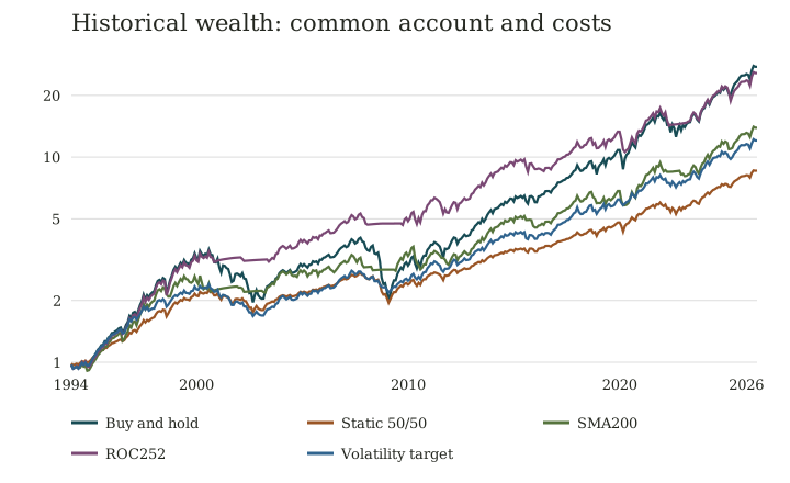
Figure 7. actual simulated month-end wealth at 5 bp for a selected comparison set, with an initial value of one. The logarithmic axis makes proportional growth comparable. All rules, not just these displayed lines, remain in the tables and companion. Month-end plotting does not reproduce every daily drawdown.
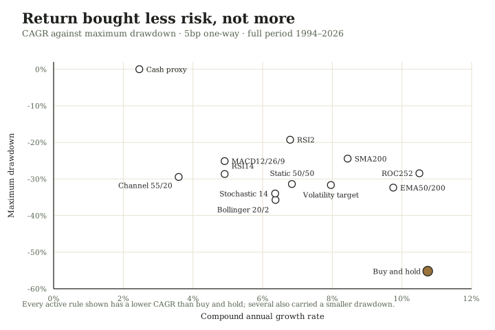
Figure 8. the same thirteen rows as the table above, plotted as return against risk. Every active rule sits left of buy and hold on CAGR; several also sit above it on drawdown.
Cost stress:25 bp one-way
| Construction | CAGR | Volatility | Max drawdown | Rebalances |
|---|---|---|---|---|
| Buy and hold | 10.74% | 18.78% | -55.19% | 1 |
| Cash proxy | 2.46% | 0.13% | 0.00% | 0 |
| Static 50/50 | 6.82% | 9.23% | -31.42% | 390 |
| SMA200 | 7.01% | 12.22% | -28.75% | 215 |
| EMA50/200 | 9.56% | 14.02% | -32.63% | 29 |
| MACD12/26/9 | 0.57% | 11.21% | -44.25% | 686 |
| ROC252 | 9.83% | 13.97% | -29.31% | 99 |
| Channel 55/20 | 2.57% | 9.18% | -31.94% | 160 |
| RSI14 | 4.41% | 10.04% | -28.80% | 78 |
| RSI2 | 1.69% | 9.84% | -33.54% | 796 |
| Bollinger 20/2 | 4.47% | 12.68% | -38.84% | 293 |
| Stochastic 14 | 2.80% | 12.90% | -41.45% | 553 |
| Volatility target | 6.99% | 10.30% | -33.22% | 6137 |
The fast MACD and RSI2 constructions show why execution assumptions belong inside the result. MACD's CAGR fell from 4.91% to 0.57%; RSI2 fell from 6.79% to 1.69%. Their formulas did not change. Their frequent state changes made a larger cost assumption economically consequential. These are comparisons of the declared simulations, not measurements that historical SPY always cost 25 bp to trade.
The volatility target rebalanced more than 6,000 times, but many adjustments were small. Counting orders alone is therefore not a complete measure of cost; traded notional and turnover matter. Conversely, a low trade count does not eliminate gap, concentration, or model risk.
Chronological slices at 5 bp
These slices describe the same continuously operated accounts. They are not fresh holdouts. No rule is retuned or replaced within a slice. The complete cost-by-period grid is retained in the downloadable results.
1994–2006
| Construction | CAGR | Volatility | Max drawdown |
|---|---|---|---|
| Buy and hold | 10.56% | 17.45% | -47.52% |
| Cash proxy | 3.91% | 0.10% | 0.00% |
| Static 50/50 | 7.46% | 8.68% | -24.03% |
| SMA200 | 9.08% | 12.70% | -22.82% |
| EMA50/200 | 12.30% | 13.69% | -21.09% |
| MACD12/26/9 | 4.85% | 11.05% | -24.47% |
| ROC252 | 12.91% | 13.85% | -19.03% |
| Channel 55/20 | 3.46% | 9.65% | -29.45% |
| RSI14 | 5.46% | 8.28% | -19.49% |
| RSI2 | 8.71% | 9.28% | -14.50% |
| Bollinger 20/2 | 8.03% | 10.58% | -31.69% |
| Stochastic 14 | 8.49% | 11.18% | -24.92% |
| Volatility target | 7.67% | 10.23% | -31.66% |
2007–2016
| Construction | CAGR | Volatility | Max drawdown |
|---|---|---|---|
| Buy and hold | 6.88% | 20.84% | -55.19% |
| Cash proxy | 0.67% | 0.09% | 0.00% |
| Static 50/50 | 4.06% | 10.14% | -31.38% |
| SMA200 | 5.08% | 11.52% | -24.43% |
| EMA50/200 | 6.78% | 12.92% | -18.07% |
| MACD12/26/9 | 2.79% | 11.98% | -25.12% |
| ROC252 | 6.75% | 13.60% | -19.82% |
| Channel 55/20 | 1.69% | 8.52% | -16.43% |
| RSI14 | 3.45% | 10.79% | -17.17% |
| RSI2 | 6.31% | 10.93% | -17.75% |
| Bollinger 20/2 | 3.37% | 14.37% | -35.72% |
| Stochastic 14 | 5.11% | 15.03% | -33.97% |
| Volatility target | 5.48% | 10.43% | -24.02% |
2017–July 2026
| Construction | CAGR | Volatility | Max drawdown |
|---|---|---|---|
| Buy and hold | 15.22% | 18.23% | -33.72% |
| Cash proxy | 2.40% | 0.12% | 0.00% |
| Static 50/50 | 8.99% | 8.96% | -17.65% |
| SMA200 | 11.19% | 12.17% | -19.43% |
| EMA50/200 | 9.52% | 15.47% | -32.36% |
| MACD12/26/9 | 7.27% | 10.47% | -15.37% |
| ROC252 | 11.30% | 14.48% | -28.45% |
| Channel 55/20 | 5.80% | 9.15% | -22.95% |
| RSI14 | 5.73% | 11.32% | -28.65% |
| RSI2 | 4.76% | 9.20% | -19.28% |
| Bollinger 20/2 | 7.34% | 13.33% | -28.65% |
| Stochastic 14 | 4.87% | 12.54% | -25.92% |
| Volatility target | 11.04% | 10.25% | -12.92% |
Paired uncertainty comparisons
The next table concerns annualized mean daily-return differences against buy-and-hold. It does not concern CAGR differences. Intervals use the approximate circular 20-session block bootstrap,2,000 replications, and the limitations stated in the protocol. The wider interval is a 99.5% marginal interval under a ten-comparison Bonferroni allocation; it is not an exact simultaneous guarantee.
| Rule | Mean difference | 95% interval | 99.5% interval |
|---|---|---|---|
| SMA200 | -3.13% | [-7.04%, 0.82%] | [-9.19%, 2.99%] |
| EMA50/200 | -1.68% | [-5.34%, 2.11%] | [-7.05%, 3.69%] |
| MACD12/26/9 | -6.56% | [-10.63%, -2.33%] | [-11.95%, -0.50%] |
| ROC252 | -1.00% | [-4.56%, 2.74%] | [-6.25%, 4.55%] |
| Channel 55/20 | -8.03% | [-12.98%, -3.26%] | [-14.95%, -1.49%] |
| RSI14 | -6.68% | [-11.70%, -1.72%] | [-14.06%, 0.91%] |
| RSI2 | -4.93% | [-9.93%, 0.34%] | [-12.26%, 2.58%] |
| Bollinger 20/2 | -5.01% | [-9.67%, -0.38%] | [-11.33%, 1.38%] |
| Stochastic 14 | -4.98% | [-9.39%, -0.52%] | [-12.08%, 0.73%] |
| Volatility target | -3.78% | [-6.61%, -0.71%] | [-8.20%, 0.40%] |
None of these intervals establishes positive arithmetic-mean outperformance for an active rule. Several conventional 95% intervals lie entirely below zero, but the broader family intervals are less decisive for many rules. The MACD and channel constructions remain below zero even in the displayed wider intervals under this approximation. This is evidence about these candidates and assumptions, not a proof that every MACD or channel policy must fail.
For SMA200, the companion also reports block-length sensitivity. A change in an interval under a different dependence assumption is information about the strength of the inference, not a reason to display only the most convenient version.
What this experiment supports
It supports the claim that indicator names conceal materially different exposure, turnover, and cost profiles. It supports several historical risk tradeoffs, and it supplies adverse evidence against simple return-superiority claims for the tested rules. It does not establish a universally best indicator, a currently deployable edge, or the absence of useful variants in other markets.
A reader seeking a method should begin with the objective: growth, drawdown management, execution, or another constraint. Then compare complete feasible policies. The edge chapter asks which payer, if any, the policy could access. The monthly construction that follows is a transparent educational contrast, not the winner of this expanded search.
Two random-rule controls
Two further policies were frozen before this calculation in expansion/RANDOM-PROTOCOL.md. They reuse this laboratory's SPY tape, dates, next-open fills, and costs. They were allowed to win. A random win would not have been an edge.
The iid coin-flip sets the next-open target to long or cash with equal probability at each completed close, independently of price, seed 20260911. The timing-destroyed channel keeps the Channel 55/20 multiset of long and cash days inside the evaluation window and permutes their dates with the same seed. Warm-up states are left in place.
Full period at 5 bp
| Construction | CAGR | Volatility | Max drawdown | Exposure | Trades |
|---|---|---|---|---|---|
| Buy and hold | 10.74% | 18.78% | -55.19% | 100.0% | 1 |
| Cash proxy | 2.46% | 0.13% | 0.00% | 0.0% | 0 |
| SMA200 | 8.44% | 12.19% | -24.43% | 77.1% | 215 |
| EMA50/200 | 9.75% | 14.01% | -32.36% | 80.4% | 29 |
| MACD12/26/9 | 4.91% | 11.18% | -25.12% | 50.5% | 686 |
| Channel 55/20 | 3.59% | 9.16% | -29.45% | 48.9% | 160 |
| Iid coin-flip | 1.22% | 13.42% | -55.14% | 48.9% | 4069 |
| Timing-destroyed Channel 55/20 | -0.08% | 13.21% | -51.51% | 48.8% | 4081 |
Neither random policy beat buy-and-hold. Neither beat the cash proxy. The coin-flip compounded at 1.22% with 4,069 trades; the shuffled channel compounded at -0.08% with 4,081 trades. Channel 55/20, which used the same number of long days as its shuffled cousin, compounded at 3.59% with 160 trades. Destroying the dates reduced the historical compound rate; it also multiplied turnover.
At 25 bp the same random policies compounded at -21.20% and -22.28%, with daily-close drawdowns of -99.96% and -99.97%. Cost, not a hidden chart edge, is what those paths mainly measured.
The 2007–2016 slice at 5 bp is retained because it is the inconvenient neighbor: the coin-flip compounded at 4.18%, ahead of MACD at 2.79% and the intact channel at 1.69%, and behind EMA50/200 at 6.78% and buy-and-hold at 6.88%. A named rule that loses a slice to a coin-flip has no timing boast for that slice. The coin-flip still finished the full sample well behind every named comparator except as a cost casualty.
Paired differences at 5 bp
Intervals are approximate circular 20-session block-bootstrap intervals, annualized by 252, seed 20260911. They are not CAGR intervals.
| Contrast | Mean difference | 95% interval |
|---|---|---|
| Iid coin-flip versus EMA50/200 | -8.19% | [-12.50%, -3.95%] |
| Iid coin-flip versus Channel 55/20 | -1.84% | [-6.26%, 2.74%] |
| Shuffled channel versus EMA50/200 | -9.52% | [-13.78%, -5.46%] |
| Shuffled channel versus Channel 55/20 | -3.17% | [-7.61%, 1.10%] |
The coin-flip versus EMA50/200 interval lies entirely below zero. The two contrasts against the intact channel include zero. This edition therefore does not claim that the channel's dates of exposure beat a shuffle of those dates at a conventional 95% arithmetic-mean standard. It does claim that these random policies, on this tape, are not a story in which coin flips beat the named books.
Reproduction: python3 -m unittest discover -s tests -p test_random_lab.py, then python3 books/research/random_lab.py.
A record that can be challenged
The companion retains the full precision metrics, all cost/period combinations, month-end account paths, seed, code, tests, protocol, and archived-input hashes. Data revisions can change a later reproduction. A correction should identify the changed input or assumption and retain the earlier record rather than silently replacing an inconvenient result.
Chapter 32
A Practical Construction: Monthly Equity and Cash
The preceding laboratory compared several fixed indicator policies. This chapter follows one monthly rule from its hypothesis through its complete specification. It was developed as a separate study, not selected as the winner of that comparison.
The method examined here is a long-only monthly trend filter applied to SPY, the State Street SPDR S&P 500 ETF Trust. It holds either the equity fund or cash. It does not sell short, borrow, trade options, or attempt to predict the next intraday movement. Its intended use in this book is an understandable example of systematic exposure management, not a personalized portfolio prescription.
Empirical hypotheses
H1. Some equity declines unfold slowly enough that a lagging trend filter can reduce exposure before the worst of the decline. This may fail in a gap, sudden crash, or rapid reversal.
H2. Avoiding some prolonged declines can reduce realized drawdown and volatility sufficiently to compensate a particular investor for missed gains and whipsaw losses. “Sufficiently” depends on the objective; lower risk is not automatically superior performance.
H3. The effect may survive modest costs and reasonable neighboring parameter choices. This is a question for measurement, not a consequence of the first two hypotheses.
Possible explanations include gradual adjustment to information, persistent flows, or investors' changing risk tolerance. These explanations are plausible research directions, not proved causes of the results. Historical evidence for other trend strategies motivates the test without validating this particular implementation in advance.
The complete rule
R1. Instrument and account. Use SPY as the equity instrument for the historical illustration, denominated in US dollars. Equity target is either 100% or 0%; remaining value is cash. The historical cash return is a Treasury-bill research proxy, not an actual brokerage offer. An implementation must name its own cash vehicle and record the yield and costs actually obtained.
R2. Data. Use split- and distribution-adjusted daily closes for the signal. Take the final trading-session close of each completed calendar month. Ten completed monthly observations are required; until then, hold cash. Do not mix raw closes in one month with total-return-adjusted closes in another.
R3. Signal. Let T_m be the month-end adjusted close and M_m the arithmetic mean of T_m through T_(m−9). If T_m > M_m, target equity. If T_m ≤ M_m, target cash. Equality is assigned to cash. Ten months is a fixed design choice, not a discovered optimum.
R4. Observation and order. Calculate only after the final monthly close is available. Submit a target-changing order for the following trading session's open, using a supported order type and the broker's stated cutoff. If timely data or an eligible order is unavailable, retain existing holdings and log the skipped change rather than claiming a fill that did not occur.
R5. Exposure before the fill. Existing holdings earn or lose the overnight move from month-end close to the next open. A sell signal cannot retroactively place the account in cash during that interval. Gap risk remains.
R6. Size and turnover. Rebalance only when the equity/cash target changes. Account for fees when determining shares so the purchase is funded without borrowing. An unchanged target creates no signal-driven trade. Whole-share rounding, distribution cash, and vehicle requirements may produce small differences in a real account; document them rather than silently redefining the rule.
R7. Costs. The baseline study deducts 0.05% of traded notional on each side, with a 0.25% sensitivity. A purchase and later sale incur two costs. Fund expenses already reflected in the price series are not deducted again. The cash proxy includes no separate trading charge, which can overstate a real implementation's cash return.
R8. Constraints. Do not add leverage to recover missed gains. Do not widen the universe, shorten the signal, or add an indicator merely because the last trade lost. Any such alteration is a new method requiring its own record and evaluation.
R9. Monitoring. Archive observations, targets, order submissions, executions, fees, and deviations. Reconcile the account with the expected holdings. The simulation marks at daily closes; actual intraday or liquidation losses can be larger than its reported maximum drawdown.
A worked decision
Suppose the ten completed month-end observations sum to 4,900, so the average is 490. The newest adjusted close is 510. The target is equity because 510 > 490. If the account is already in equity, there is no change. If it is in cash, the order is scheduled for the next eligible session.
If the next opening price gaps upward, the account buys at the actual opening execution, not at yesterday's close. If it gaps downward while the account is already invested, the account bears that overnight loss even if the signal has changed to cash. The rule governs action; it does not govern the available price.
Suppose a funded cash account has $10,000 and faces a one-way proportional cost c = 0.0005. Buying $10,000 of stock would leave no cash for the fee. In the continuous-unit model the purchased notional is $10,000/(1+c), approximately $9,995.00; the remainder pays the modeled cost. The research code uses this funded accounting rather than creating a small margin balance.
The purpose, fixed before looking
The principal historical objective is positive net compound growth together with lower daily-return volatility and a smaller daily-close maximum drawdown than equity buy-and-hold, in both the full sample and the combined post-2007 sample. This is a risk-management objective, not a requirement to beat SPY's return.
The comparisons include buy-and-hold, Treasury cash, and a static 50/50 equity/cash portfolio rebalanced monthly. The latter matters because lower stock exposure can reduce risk without successful timing (Proposition 27). Eight- and twelve-month filters, higher costs, zero cash income, and next-session-close execution are published as sensitivities. The ten-month rule remains the principal specification even when another lookback looks better afterward.
What would count against the method
Failure to retain positive growth or reduce the specified risks in the declared windows counts against its stated historical objective. Dependence on implausible fills or negligible costs also counts against it. Underperformance to the static mixed portfolio is evidence that the extra operational burden may not be worthwhile for the relevant period and objective.
Even a passing result supports only a bounded statement about a historical simulation. It does not establish an investable edge for all accounts, superior after-tax wealth, protection against all crashes, or an acceptable personal drawdown. The next chapter reports what the fixed test actually found.
Chapter 33
What the Historical Test Found
The method passed its declared historical risk-reduction objective against fully invested SPY. It did not establish that timing was superior to simpler allocations, and it did not earn the highest return. The distinction is the result, not a footnote.
The objective and parameters were recorded before this calculation according to the research log. They were not independently preregistered. The sample and strategy family were selected retrospectively in September 2026; the post-2007 period is post-publication history, not a newly untouched prospective test.
Data, execution, and limits
The sample runs from January 3, 1994 through July 31, 2026. Earlier SPY observations supply the signal warm-up. It uses Yahoo Finance daily open, close, and adjusted-close observations retrieved September 5, 2026. Adjusted open equals raw open multiplied by that day's adjusted-close/raw-close ratio. Existing equity earns the previous adjusted close to the next adjusted open; changed holdings then earn the adjusted open to close. Dividends are not added again.
This is a vendor-adjusted total-return simulation, not an exact share ledger with dividend payment dates. Adjusted data can be revised. SPY's fund operating expenses are embedded; the model additionally charges 0.05% per one-way traded notional. It begins in cash and pays the initial entry cost. It does not charge a final liquidation, model taxes, or adjust for inflation.
Cash uses Kenneth French's monthly RF research returns. Each realized monthly return is allocated geometrically over that month's equity trading sessions, half overnight and half intraday. This retrospective synthetic accrual is not a rate known at the start of every day or an available cash-account return. It is not used to choose the signal. The zero-cash-income sensitivity shows how much the modeled interest contributes, but neither case substitutes for an actual cash vehicle's ledger.
CAGR uses elapsed calendar time. Volatility is the sample standard deviation of daily returns multiplied by the square root of 252. Drawdown is measured at daily closes, so it can miss larger intraday losses. Subperiods retain the holdings from the continuous simulation while resetting the reporting high-water mark. All returns are nominal; 2026 is partial through July.
Full-period comparison
| Strategy | CAGR | Volatility | Maximum drawdown |
|---|---|---|---|
| 10-month filter | 9.54% | 12.84% | -24.79% |
| SPY buy-and-hold | 10.83% | 18.76% | -55.19% |
| Static 50/50, monthly rebalanced | 6.88% | 9.22% | -31.38% |
| Cash proxy | 2.46% | 0.13% | 0.00% |
The filter's lower drawdown came with a lower compound return than buy-and-hold. It held equity on roughly 78% of daily closing observations. Holding less equity explains some reduction in risk; the result alone does not establish timing skill. The static 50/50 allocation had lower volatility but a larger full-period maximum drawdown than the filter.
The principal filter made 47 nonzero rebalances including its initial entry. Its worst month was August 1998, about −14.12%; its worst calendar year was 2022, about −21.06%. The longest observed period below its prior high lasted 1,001 calendar days. At the final observation it remained below its latest high. These are substantial costs of the method even though it passed its declared comparison with fully invested equities.
Fixed historical slices
1994–2006
| Strategy | CAGR | Volatility | Maximum drawdown |
|---|---|---|---|
| 10-month filter | 12.07% | 12.97% | -19.03% |
| SPY buy-and-hold | 10.77% | 17.41% | -47.52% |
| Static 50/50, monthly rebalanced | 7.56% | 8.65% | -24.03% |
2007–2016
| Strategy | CAGR | Volatility | Maximum drawdown |
|---|---|---|---|
| 10-month filter | 7.28% | 12.90% | -20.12% |
| SPY buy-and-hold | 6.88% | 20.84% | -55.19% |
| Static 50/50, monthly rebalanced | 4.06% | 10.14% | -31.38% |
2017–July 2026
| Strategy | CAGR | Volatility | Maximum drawdown |
|---|---|---|---|
| 10-month filter | 8.55% | 12.62% | -24.79% |
| SPY buy-and-hold | 15.22% | 18.23% | -33.72% |
| Static 50/50, monthly rebalanced | 8.99% | 8.96% | -17.65% |
Combined post-2007
| Strategy | CAGR | Volatility | Maximum drawdown |
|---|---|---|---|
| 10-month filter | 7.90% | 12.76% | -24.79% |
| SPY buy-and-hold | 10.87% | 19.61% | -55.19% |
| Static 50/50, monthly rebalanced | 6.44% | 9.58% | -31.38% |
The 2017–July 2026 comparison is especially important: static 50/50 earned a higher CAGR than the filter while showing lower volatility and a smaller drawdown. That observation prevents a claim that the extra timing decisions consistently improved the tradeoff.
In the full sample, the ten-month filter underperformed buy-and-hold in approximately 57.8% of the 332 overlapping sixty-month windows. In the post-2007 slice it underperformed in approximately 88.1% of such windows. Overlapping windows share data and are descriptive observations, not independent statistical trials. The method can demand patience without rewarding that patience relative to the benchmark.
Sensitivities, not replacement winners
| Strategy | CAGR | Volatility | Maximum drawdown |
|---|---|---|---|
| 8-month filter | 10.25% | 12.35% | -24.79% |
| 10-month filter | 9.54% | 12.84% | -24.79% |
| 12-month filter | 10.44% | 12.95% | -22.27% |
| 10-month filter, 0.25% one-way cost | 9.23% | 12.85% | -25.69% |
| 10-month filter, zero cash income | 9.02% | 12.84% | -25.85% |
| 10-month filter, next-session close | 9.66% | 12.89% | -26.61% |
The neighboring lookbacks had favorable full-sample results under the specified risk objective, but some outperformed the principal ten-month choice. We retain the original choice and show the alternatives rather than relabeling the best historical parameter as the method discovered by proof. The larger one-way cost reduced the principal CAGR. Zero cash income also reduced it. Next-session-close execution changed the path and drawdown.
The accompanying research tables retain every declared sensitivity in every fixed period, including higher-cost versions of the neighboring filters and benchmarks. The manuscript table is a summary, not a selection of the only results that were calculated. Cash-excess Sharpe ratios are in the full tables; the zero-cash scenario uses a zero reference and should not be compared as if it used the same RF benchmark.
What “works” means here
The supported claim is specific: in this retrospective, cost-adjusted simulation, the rule retained positive growth and reduced daily volatility and maximum daily-close drawdown relative to SPY buy-and-hold in the full and post-2007 intervals. A trader seeking that particular tradeoff has a concrete candidate to examine.
The unsupported claims would be that this proves positive future expectancy, that it beats buy-and-hold or a static mixed portfolio generally, that it is optimal, or that a monthly average prevents catastrophic losses. There are no confidence intervals, dependence-robust significance tests, or estimates of the timing covariance in Proposition 26 here. These descriptive results do not establish a statistically validated edge.
Published work by Faber supports studying a monthly average; research by Moskowitz, Ooi, Pedersen, and Hurst supports studying trend strategies across other markets. Those are distinct studies with distinct data and assumptions. They do not convert this simulation into a theorem or independently replicate its exact implementation.
The later public record is similarly mixed rather than uniformly confirmatory. Asness, Moskowitz, and Pedersen document multi-asset value and momentum premia; Barroso and Santa-Clara show that risk-managed equity momentum improved a historical Sharpe ratio while leaving crash risk smaller but not zero. Huang, Li, Wang, and Zhou find little asset-by-asset time-series predictability in the original futures sample. McLean and Pontiff, Hou, Xue, and Zhang, and Novy-Marx and Velikov show that many published predictors shrink after publication, fail stricter reconstructions, or do not survive costs. This laboratory is one specified SPY/cash rule. It inherits none of those papers' tables and supplies none of their missing replications.
The appropriate next step is prospective operational verification and a comparison with the simpler alternative the trader could actually hold. If the objective is consistently superior return at comparable risk, this study has not established it. If the objective is a transparent rule with a demonstrated historical reduction in equity drawdown and volatility, the study supplies evidence with clearly visible limits. That is the sense in which a benchmark loser can still be doing the work it was hired to do. The inference chapter separates that case from a convention loser and from a selected winner.
Reproduction
The research companion includes the protocol, Python standard-library calculation, focused accounting and timing tests, source URLs, input hashes, and complete numerical tables. Run python3 books/research/backtest.py in the source project to reproduce the archived-input calculation. The public companion explains how to retrieve inputs separately; later vendor downloads may differ from this edition's hashes.
Research companion: https://kuttystauder.com/book-assets/trader-research.zip.
Chapter 34
The Discipline of Operation
A trading rule turns available observations into instructions. Your task is to record those observations and execute the instructions consistently enough to compare the actual account with the stated method. The process below applies to a monthly allocation, an intraday strategy, or another complete specification; the monthly example shows how to keep the ledger concrete.
A strategy worksheet
Complete this before collecting a new performance result. If an answer is missing, record it as an unresolved research decision; do not let the backtest choose it silently.
| Field | What to write |
|---|---|
| Objective and comparison | The outcome you want to improve and the simpler policy you could otherwise follow |
| Market and universe | Exact instruments, historical eligibility, session, timezone, and contract or corporate-action treatment |
| Information clock | What is known at each decision, its source, warm-up, revisions, and missing-data response |
| Entry and exit | Direction, trigger, order type, equality cases, cancellation, stop, and final exit |
| Size and financing | Account or position risk budget, quantity rounding, exposure caps, margin or borrow, and fee funding |
| Net accounting | Fees, spread, slippage, financing, cash return, and exclusions such as tax |
| Evidence plan | Development and evaluation periods, all variants, benchmarks, and uncertainty calculation |
| Pause and rejection rules | Operational faults that stop new orders; economic evidence that would reject the claim |
| Review and version | Review dates, rule version, and a record of what changed and why |
For a first worked completion, use the monthly rule and its reported limitations. For ORB, choose either the stock specification or the futures specification in the special study; mixing their selection, exits, or sizing creates another experiment.
From a worksheet to a decision
First, check that the necessary historical inputs exist. Then replay a few individual decisions by hand, including a loss, a gap, and a missing-data case. Confirm that the code follows the written rule before interpreting its total profit. Run the frozen comparison and retain every declared variant.
Afterward, choose one of three research responses. Reject the current claim if the fair comparison fails its stated objective. Revise the specification if a concrete data or implementation error explains the failure, preserving the old record. Continue with prospective paper observation if the historical evidence is sufficiently relevant to justify that next test. A favorable backtest alone does not determine whether to commit live capital.
Before considering capital
Run the rule in a prospective paper ledger. This means recording signals as they become available, not reconstructing them after the market has moved. Verify the trading calendar, the required completed observation, the order cutoff, the next execution price, and the treatment of cash and instrument-specific obligations. A paper profit does not prove an edge, but a broken paper ledger is sufficient reason to repair operations before exposing capital.
Keep money needed for near-term obligations outside the experiment. The monthly filter provides no guaranteed maximum loss. A person who cannot tolerate the demonstrated drawdowns or long benchmark shortfalls has learned something useful from the study; there is no need to reinterpret discomfort as a philosophical failure.
Why day trading is not a viable livelihood for most people
Day trading should not be presented as a dependable way for an ordinary household to meet its expenses. Belief does not establish positive expectancy, and repeated participation does not guarantee learning. Practice can improve execution; it cannot make a rule profitable merely by making its execution consistent. The relevant questions concern the probability and size of outcomes, costs, uncertainty about the edge, and the capital available when losses arrive.
The historical evidence is severe, although its scope must remain visible. Barber, Lee, Liu, and Odean studied Taiwan stock-market day traders during 1992–2006. Fewer than 1% reliably earned positive abnormal returns after fees. This is a finding about persistent performance, not the proportion who ever had a profitable year. The study also identifies persistent differences in skill, supporting the existence of a small successful group. Published paper.
Chague, De-Losso, and Giovannetti's June 2020 working paper examined new Brazilian equity-futures day traders. Among the 1,551 who traded for more than 300 days, 97% lost money after exchange and brokerage fees. Their regressions found no evidence of learning among persistent traders. The percentage describes that subgroup, not every entrant; taxes, platform costs, and course expenses were excluded. Authors' manuscript.
These studies do not measure every market, every person, or every sophisticated method. They do justify rejecting the promise that sufficient commitment usually produces a trading livelihood. They do not establish that inadequate capital caused most failures. Capital adequacy is a separate constraint, which the following arithmetic explains.
An edge and enough capital are different requirements
A positive average outcome is compatible with a sequence of losses. Several positions may lose together; execution may worsen precisely when prices move fastest. A stop limits an intended loss under a fill assumption. It does not guarantee that fill or guarantee a maximum account drawdown. A household can run out of usable capital before an uncertain long-run advantage has time to appear.
Consider a simplified stress scenario. Let B mean starting trading capital, d a loss equal to a fraction of that starting capital, w the monthly withdrawal, m the number of months, and M the capital that must remain available. The condition is:
B × (1 − d) − m × w ≥ M.
In words: after the assumed trading loss and the withdrawals, enough money must remain to continue. Rearranging the same condition gives:
B ≥ (M + m × w) / (1 − d).
Suppose the scenario assumes a 30% trading loss, six withdrawals of $3,000, and a requirement to retain $10,000. It requires at least ($10,000 + $18,000) / 0.70 = $40,000 at the start. A $25,000 account would have only $17,500 after the assumed trading loss, less than the $18,000 withdrawals alone.
This is an illustration, not an estimate of safe starting capital. It defines the trading loss as a fraction of starting capital; actual loss and withdrawal timing changes the path. A larger drawdown, longer drought, higher margin requirement, or loss of the estimated edge can invalidate the chosen scenario. More capital can absorb more adverse outcomes; it cannot turn negative expectancy positive.
A practical plan therefore separates household reserves from trading capital, states the drawdown and withdrawal assumptions, and identifies the point at which trading must stop. If the household requires dependable monthly income, an irregular and uncertain trading return may fail that requirement even when a historical backtest is profitable. Reducing position size helps preserve the account but also reduces the dollars available for living expenses.
What the skilled minority must demonstrate
The evidence permits the possibility of durable skill. It does not make sophistication a certificate of profitability. A sophisticated trader still needs evidence that the proposed advantage survives realistic execution, costs, changing conditions, and evaluation on observations that did not determine the rule. Sound risk management makes exposure more survivable; it does not supply the missing advantage.
Understanding causes means stating an explanation that can be investigated: why an order-flow imbalance might persist, which participants could create it, when it should disappear, and what observations would contradict it. A plausible explanation remains a hypothesis until the trading rule earns relevant empirical support. Understanding probability also means accepting that even a supported explanation cannot specify the next outcome with certainty.
The practical conclusion is to assess three requirements separately: an executable net advantage, resources sufficient for adverse paths, and compatibility with the trader's obligations. Failure of any one is enough to make a method unsuitable. The strategy worksheet records those requirements before enthusiasm is allowed to stand in for evidence.
A passed prop-firm challenge does not replace those three requirements. Passing is a path through a purchased knockout. It is not household income and not a measurement of the instrument’s mean. Write the knockout sheet in the prop-firm chapter if that is the game being played; do not import Combine dollars into this ledger as if they were capital.
The decision ledger
For every method, retain the signal inputs, intended action, actual action, fill, quantity, costs, resulting position, and any departure from the rule. Include skipped trades and the reason for skipping them. Keep a version identifier so a later change cannot silently rewrite an earlier decision.
For the monthly example, record the date and provider of the ten observations. Record their average, the final comparison, the old target, the new target, and whether a trade was required. Record the time the data became available and the time the order was submitted. Finally record the fill, fee, actual cash return, and any reason the account differs from the modeled holdings.
If the signal was equity but an outage prevented the purchase, record a missed execution. Do not rewrite the ledger as though the strategy had been in equity. If an order filled poorly, include that cost. A record that excludes operational failures describes an imaginary account.
Three different failures
An execution failure occurs when the intended rule was not carried out: wrong data, late order, incorrect share size, or an unrecorded fee. Correct the process and retain the cost in the historical record.
A model failure occurs when the assumptions or performance claims no longer describe what the method produces. It cannot be diagnosed from every isolated loss. But neither can it be dismissed indefinitely by claiming that an unseen edge will eventually reveal itself. Compare realized behavior with the declared objective and alternatives at scheduled reviews.
A fit failure occurs when the rule's demonstrated behavior is incompatible with the user's needs. The method can behave exactly as tested and still be unsuitable. Someone requiring reliable short-term cash withdrawals faces a different problem from someone able to accept years of benchmark underperformance.
These failures require different responses. A missed order is not repaired by inventing a new indicator. A vanished return effect is not repaired by greater devotion. An unsuitable objective is not repaired by calling the investor weak.
A review calendar
Check operations after each scheduled decision. Set the economic review schedule before the experiment, at a frequency appropriate to its horizon and available observations. For the monthly example, a fixed annual review avoids redesigning the rule after every uncomfortable month. An intraday ledger needs session-level operational reconciliation; that does not make each day enough evidence for a new economic conclusion. Include all observations, costs, departures from the rule, and the same benchmarks used at the beginning. If the account's cash return differs materially from the research proxy, recompute the comparison with the actual rate.
A review may conclude that the rule should remain unchanged, be suspended, or be replaced by a simpler allocation. Suspend immediately when data or order integrity is in doubt; there is no requirement to continue an operationally invalid experiment until the annual date. Resume only after the cause is understood and the account reconciled.
If redesign is needed, keep the prior record intact. Specify the new hypothesis, freeze its rules, and label the next experiment separately. Do not splice the best periods of successive strategies into a composite that no one could have followed at the time.
The place of affect
Fear may signal a real risk, a mismatch between size and resources, or a misleading response to noise. Confidence may reflect understanding or merely a recent winning streak. Neither affect carries its own certificate of truth.
The Spinozan exercise is to investigate what the affect is doing to the decision. Is the urge to increase size a response to stronger evidence, or a desire to erase a loss? Is the urge to abandon the rule based on a broken premise, or on seeing another strategy's recent gain? Write the distinction before acting.
This does not make a person emotionless. Spinoza recognizes active joy and desire as well as passive affects (Ethics III, propositions 58–59). There can be satisfaction in accurate accounting, restrained exposure, and a conclusion honestly revised. The account need not rise every month for those activities to have value.
The truth of trading
The truth established by the proofs is conditional and demanding. Outcomes must be measured net of costs. Capital compounds. Loss and recovery are asymmetric. Estimated probabilities are not known probabilities. Information must precede action. A finite history does not command its own continuation.
The empirical truth is narrower: a particular historical simulation produced a particular set of gains, losses, and tradeoffs. It is enough to study that result seriously without turning it into a promise. A useful method is one whose rules can be executed and whose claims remain proportionate to its evidence.
The trader's freedom is not exemption from uncertainty. It is the ability to act within uncertainty without falsifying it. Keep the premises visible. Keep the ledger intact. Let the result correct the story.
Primary references and research record
- Euclid, Elements, Book I: definitions, postulates, common notions, and propositions. The proof architecture is the inspiration, not a claim that markets satisfy Euclidean postulates. https://mathcs.clarku.edu/~djoyce/elements/bookI/bookI.html
- Spinoza, Ethics, especially III definitions 1–3, propositions 1, 6–7, 58–59. Contemporary trading applications are this author's interpretations. https://www.gutenberg.org/ebooks/3800
- Kelly, J. L. (1956), “A New Interpretation of Information Rate.” Expected logarithmic growth and the distinction from expected wealth. https://doi.org/10.1002/j.1538-7305.1956.tb03809.x
- Faber, M. (2007; updated 2013), “A Quantitative Approach to Tactical Asset Allocation.” The author-hosted version specifies a ten-month moving-average model and discusses historical limitations. Its original execution and cost assumptions differ from this edition's test. https://mebfaber.com/wp-content/uploads/2016/05/SSRN-id962461.pdf
- Moskowitz, T. Ooi, Y. and Pedersen, L. (2012), “Time Series Momentum.” Evidence across futures and forwards; not a direct validation of the single-ETF rule here. https://www.aqr.com/Insights/Research/Journal-Article/Time-Series-Momentum
- Hurst, B. Ooi, Y. and Pedersen, L. (2017), “A Century of Evidence on Trend-Following Investing.” Reconstructed diversified trend strategies differ from this book's implementation. https://www.aqr.com/-/media/AQR/Documents/Insights/Journal-Article/AQR-JPM-Fall-2017.pdf
- State Street, SPY fund information. Instrument identity and inception; this fund tracks large-cap US equities, not the entire global opportunity set. https://www.ssga.com/us/en/intermediary/etfs/state-street-spdr-sp-500-etf-trust-spy
- Yahoo Finance, historical price adjustments. Vendor-adjusted data are revisable and do not supply an exact dividend-payment-date ledger. https://help.yahoo.com/kb/SLN28256.html
- Kenneth French data library, factor definitions and RF series. Research Treasury-bill returns are used as a cash proxy with an explicitly synthetic daily accrual convention. https://mba.tuck.dartmouth.edu/pages/faculty/ken.french/Data_Library/f-f_factors.html
- This edition's research protocol, code, tests, and numerical tables: https://kuttystauder.com/book-assets/trader-research.zip. Local archived input checksums identify the run; source data can change on later retrieval.
Chapter 35
Strategy Blueprints, Research Templates, and Rejection Rules
The monthly equity/cash method, the daily laboratory rules, and the Donchian-gated opening-drive have actual retrospective results in this edition. Blueprints 1, 4, and 10 summarize those complete rules; their protocols supply the precise calculation and execution conventions. The other seven constructions are research templates. They identify the decisions an investigator must make, and sometimes illustrate particular parameter choices, but they are not directly executable specifications or tested recommendations.
The common contract is explicit information timing, an eligible universe, a position rule, sizing, execution, costs, risk constraints, and rejection criteria. Before testing a template, record every missing value in a dated protocol: instruments, estimation windows, risk budgets and caps, order conventions, cost assumptions, and failure rules. A template with unresolved choices is not yet a complete trading method. Choosing those values after inspecting performance creates another round of model selection.
Blueprint 1: slow equity trend with a risk objective
Evidence status: tested retrospectively in this edition's original monthly study.
Use SPY adjusted month-end closes. Compare the latest close with the mean of the latest ten completed month-end closes. Target 100% SPY when strictly above and cash otherwise. Calculate only after the month closes; fill at the next eligible open. Rebalance on state changes, with no leverage or shorting. Use the documented cash and cost assumptions when reproducing the book, and replace them with actual account conventions when assessing an implementation.
The declared objective is positive historical growth with lower volatility and drawdown than fully invested equities over the specified comparisons. It is not maximum CAGR or universal superiority. Compare against buy-and-hold and a static lower-exposure portfolio. Reject claims of superiority that disappear under those comparisons; pause operational use when inputs, order timing, or actual costs cannot be reconciled with the rule. The original study's limitations remain attached to the blueprint.
Research template 2: a diversified time-series momentum research portfolio
Evidence status: related historical literature exists; this exact blueprint is not tested here.
Freeze an eligible list of liquid futures contracts before evaluation, with contract multipliers, first-notice/last-trade rules, and a roll schedule that avoids delivery. At each month-end, compute twelve-month past excess returns for each instrument using the actual contract-return convention. Set direction by the sign, then scale each preliminary exposure inversely to a trailing volatility estimate calculated from eligible past daily returns. Normalize the portfolio to a declared risk target, with explicit per-contract and gross-leverage caps. Fill after the signal using specified next-session orders and roll costs.
The research must retain instruments that later disappear and must not infer contract P&L from a continuous chart alone. Compare with passive risk-matched exposures and simpler constant allocations. Stress correlated reversals, margin increases, and missed rolls. Reject the construction if its historical edge depends on unavailable fills, optimistic roll treatment, or leverage that its funding plan cannot sustain. Literature support for the family does not certify these exact windows and caps.
Research template 3: long-only cross-sectional momentum
Evidence status: family literature exists; the following template is untested here.
At each month-end, form a point-in-time universe of U.S. common shares on the chosen eligible exchanges. For a research example, require a closing price of at least 5 dollars and trailing 60-session average dollar volume of at least 10 million dollars; rank the 500 most liquid eligible names. These thresholds are design choices, not universal liquidity standards. Rank their cumulative returns from twelve months ago through one month ago, excluding the most recent month. Equal-weight the top 50 at the next session's declared execution benchmark, with no shorting or leverage. Missing eligible history removes a name before ranking; retain cash if fewer than 50 qualify under the frozen rule.
Include delistings, corporate actions, actual historical membership, turnover, and taxes only if the stated study models them. Compare with the same eligible universe equally weighted and with factor-aware benchmarks. Stress momentum reversals and concentration by sector. Reject if the result survives only in today's survivors or relies on trading illiquid constituents at closing midprices.
Blueprint 4: short-horizon equity reversion
Evidence status: the exact SPY RSI2 variant is tested in the laboratory.
Use Wilder RSI2 from completed adjusted closes, with the specified seed. In cash, enter when RSI is strictly below 10; while long, leave when RSI is strictly above 50. Otherwise retain state. Execute at the next adjusted open, target either 100% SPY or cash, and include both cost assumptions. No intraday stop is inferred from a daily bar.
The research question is not whether RSI2 can identify a low number. It is whether this specific reversal policy offers an acceptable net risk–return tradeoff relative to cash, buy-and-hold, and a lower-exposure alternative. The laboratory's cost stress is part of the answer. Reject a low-cost performance claim when the reader's realistic all-in costs are closer to the adverse scenario and the resulting economics no longer meet the declared objective.
Research template 5: an economically selected pair
Evidence status: a research blueprint, not a tested recommendation.
Choose the eligible economic relationship before looking at the proposed trading interval. Use a fixed historical formation window to estimate a hedge and residual distribution, then freeze those estimates for a subsequent trading block. A concrete example uses 252 formation sessions and a 63-session evaluation block. Enter a spread position when the residual exceeds±2 formation-standard-deviation units; close when it crosses zero, at the end of the block, or when a separately declared model/financing stop occurs. Order both legs using a specified synchronized execution process. Include actual borrow eligibility and costs for the short leg.
Do not increase exposure merely because a deviation grows. Set gross notional, single-name, sector, and financing limits before evaluation. Compare against random or economically comparable pairs selected by an equally explicit procedure. Reject the pair when the relationship has changed, the hedge depends on future fitting, or the position cannot survive plausible basis widening and borrow recall. The numerical thresholds here define an experiment; they do not prove a stationary spread.
Research template 6: defined-risk event optionality
Evidence status: a payoff-analysis blueprint, not a historical performance claim.
Choose a specified event and a listed European-style or otherwise carefully modeled option structure with a contractually bounded maximum loss. Record the contract, expiry, strike, multiplier, bid/ask entry price, settlement, and exercise terms. For a long straddle example, compute expiry breakevens from the total premium and financing convention. Forecast a distribution of event outcomes using information available before the order, then compare expected payoff with the executable premium and costs. Fix whether the position is held to expiry or exited after the event; an early exit requires a model of remaining implied volatility and spreads.
Cap premium at a preselected research budget and model a full premium loss. Compare against no trade and a simpler underlying exposure. Reject if the claimed advantage is merely “a big move is coming,” if historical option quotes are stale or non-executable, or if the forecast ignores the option price. A bounded loss helps define risk; it does not make the expectation favorable.
Research template 7: collateral-aware cash-and-carry
Evidence status: the matched-payoff identity is proved; no live opportunity is asserted.
Select an identical deliverable spot asset and dated derivative with enforceable common settlement. Record spot ask, derivative bid, all financing terms, custody, delivery, transfer, and fees. Calculate terminal net payoff and a pathwise collateral plan under specified basis and volatility shocks. Enter only if the stated economic threshold and financing constraints are both met. Hold or unwind according to the recorded contract plan; do not substitute a perpetual without rewriting the funding and basis analysis.
Compare the available net spread with a risk-free or low-risk alternative that uses the same capital and liquidity assumptions. Reject when the apparent spread is compensation for an unmodeled obligation, when transfers are unreliable, or when adverse variation margin would force premature liquidation. A positive terminal identity before costs is not sufficient.
Research template 8: execution improvement without an investment forecast
Evidence status: conditional execution mathematics is proved; venue-specific parameters require measurement.
Take a pre-existing buy or sell decision with fixed quantity, arrival time, deadline, and price constraints. Compare a constant-rate schedule, a forecast-volume schedule, and a declared participation cap using the same eligible market data and order types. Measure implementation shortfall, fill rate, opportunity cost, fees, and adverse markouts. Estimate any impact model only from permitted earlier observations, and retain an operational fallback for stale data or venue failure.
The objective is to improve implementation, not predict investment returns. Reject a schedule whose apparent savings require future volume, fictitious queue fills, or unrecorded urgency changes. This blueprint can be useful even when the investment itself has no directional edge; it reduces the cost of carrying out an independently justified decision.
Research template 9: a Turtle-style futures unit book
Evidence status: Faith's rules are sourced; later multi-asset trend papers exist; this exact book is not tested here.
Freeze an eligible liquid futures list, multipliers, roll calendar, and correlation groups before evaluation. Compute N as Faith's 20-day ATR with a stated seed. Size a Unit so that one N equals 1% of working equity. Trade System 2, or a declared mix with System 1 including the skip-last-winner bookkeeping and 55-day failsafe. Add units every ½N from the prior fill, cap at four units per market and at the declared group and directional limits, and place 2N stops with the stated lift rule. After a 10% loss from working notional, cut that notional by 20% until the restore rule fires. Include roll costs, daily limits, and a gap-through-stop assumption.
Compare with a passive risk-matched futures allocation and with this edition's monthly equity/cash filter. Stress a 1987-style correlated shock and a long non-trending window. Reject any claim that copies Faith's 80% recollection or Hurst's 1880–2013 Sharpe ratio onto this untested specification. See the Turtle chapter and the risk worksheet.
Blueprint 10: Donchian-gated opening-drive on a daily index
Evidence status: tested retrospectively in this edition; the declared edge gate failed.
Use the archived SPY daily series and the laboratory Channel 55/20 state. Trade a same-session long only when yesterday's channel state is long. The trigger is today's open plus 10% of prior ATR(14); the stop is 10% of that ATR below the fill. Exit survivors at the close. Assume the stop whenever the same daily bar can also print it. Skip a session when that stop cannot cover a round-trip at the declared one-way cost. Hold cash overnight.
Compare the gated rule with buy-and-hold, the cash proxy, overnight Channel 55/20, and the same opening-drive without the Donchian gate. Reject any transfer of Zarattini's stock-ORB table or Faith's Turtle recollection onto this daily analogue. The edition's calculation did not beat the overnight channel or buy-and-hold after 5 bp costs. The frozen protocol is books/research/expansion/SPINOZAN-ORB-PROTOCOL.md in the research companion. Results are in the special study.
Choosing among the blueprints
Do not select by the most attractive historical curve alone. Begin with the information you can obtain, the instrument mechanics you understand, the costs you can actually achieve, and the risk objective you intend to serve. Eliminate methods whose assumptions cannot be met. Then evaluate the remaining complete policies against simpler alternatives.
The most impressive method is not the one with the most conditions. It is the one whose conditions are explicit, whose evidence survives adverse comparisons, and whose operator can identify a failure before explaining it away.
An externally studied intraday case
The five-minute opening-range examination complements these blueprints with a published stock study and six original conditional demonstrations. Its stock portfolio results are externally sourced. The separate NQ pilot is a limited public-data replay with declared deviations, not a replication of the stock portfolio. The special study separates the historical rule from a proposed trailing-exit comparison and from any futures adaptation.
Chapter 36
The Indicator and Strategy Atlas
This atlas is a map to the arguments, not a league table. “Proved” means the stated mathematical property has a demonstration in this edition. “Historical evidence” means an identified study or the laboratory supports a bounded claim. “Untested here” means no performance estimate has been manufactured for that construction.
Price and trend tools
| Tool or family | What it measures | Strongest defensible use and principal limit |
|---|---|---|
| SMA, EMA, weighted averages | A weighted memory of price | Transparent state/filter construction; lag and noise tradeoffs depend on the path |
| MACD, PPO | Difference between fast and slow memories, optionally normalized | Momentum representation; agreement with its defining EMA ordering is redundant |
| ROC, price momentum | Endpoint price change or return | Continuation feature; does not choose a profitable horizon |
| Donchian channels | Past high/low extrema | Repeatable breakout states; current-bar inclusion can make a strict breakout impossible |
| Percentage filters | Movement from evolving extrema | Explicit path-dependent state; not equivalent to a fixed-window return |
| ADX/+DI/−DI | Smoothed directional-movement relationships | Strength/direction decomposition; ADX alone has no directional sign |
| Parabolic SAR | A stateful accelerating exit reference | Consistent exit construction; fill and reversal conventions matter |
| Ichimoku | Extrema midpoints and displaced displays | Multi-horizon organization; display time must not replace input time |
| Adaptive averages | State-dependent smoothing coefficients | Potential responsiveness control; adaptivity is not proof of optimality |
Oscillators and distance measures
| Tool or family | What it measures | Strongest defensible use and principal limit |
|---|---|---|
| Wilder RSI | Smoothed gains relative to gains plus losses | Normalized recent strength;100 can persist on a rising path |
| Fast stochastic | Close's location in a high/low window | Range-position feature; conventional thresholds do not command reversals |
| Williams %R | The same range position on a negative scale | Affine equivalent of fast stochastic under identical inputs |
| CCI | Typical-price deviation divided by mean absolute deviation and a scale constant | Deviation feature; not confined to±100, but finite-bound under the specified fixed window |
| Stochastic RSI | RSI's location in its own recent range | Extra normalization; not a new independent observation |
| Bollinger %b | Rescaled rolling z-score | Relative location; not a probability |
| Bollinger bandwidth | Band width relative to center | Dispersion-state feature; a squeeze does not choose direction |
| ATR/NATR | Smoothed true range, optionally price-normalized | Range sizing and risk context; no direction or gap-loss guarantee |
| Keltner-type channels | Center plus/minus an ATR multiple | Range envelope; exact platform formula and role must be stated |
Volume and auction tools
| Tool or family | What it measures | Strongest defensible use and principal limit |
|---|---|---|
| OBV | Cumulative volume signed by close change | Participation feature; discards return magnitude and is not exact aggressor flow |
| Accumulation/distribution | Volume weighted by within-bar close location | OHLCV compression; not a direct observation of investor cash movement |
| Chaikin money flow | Normalized accumulation/distribution over a window | Volume/location feature; denominator and flat-bar treatment matter |
| Money Flow Index | Price-times-volume classified by typical-price changes | Volume-sensitive oscillator; no inherent valuation or reversal theorem |
| VWAP/anchored VWAP | Volume-weighted executed-price or bar-typical average from a declared start | Benchmark and scenario reference; below the line is not cheap, not a trapped inventory, and not a tested reclaim edge; complete reference |
| Breadth | Participation across a defined universe | Cross-sectional context; historical membership and weighting are essential |
| Volume profile | Traded volume allocated to price bins | Auction description; does not prove future resting demand |
| Market profile | Time-price observations by bins | Auction description; time occupancy is not the same as volume |
| Trade/book imbalance | Classified trades or displayed depth | Potential short-horizon information; latency, coverage and fill conditioning dominate implementation |
Chart and structural claims
| Tool or family | Proven or exposed property | Evidence boundary |
|---|---|---|
| Candles and chart formations | Identical historical shape admits opposite continuations | Computational pattern research can find distributional information; net policy needs a separate test |
| Support/resistance | A reference event must be fixed before its revisit | Retrospective successful retests cannot estimate all first-touch outcomes |
| Fibonacci levels | Sequence identities do not determine market continuations | Anchors, scale, tolerance and comparison ratios need an empirical protocol |
| Gann angles | Independent axis rescaling changes angle | A scale-free predictive claim fails without normalization |
| Elliott counts | Scenario descriptions require fixed grammar and invalidation | No general net-profit validation supplied here; failed counts must be retained |
| Centered pivots/ZigZag | Future-confirmed extrema cannot be known at the pivot time | Useful descriptive labeling; historical trading must use confirmation time |
| Cycles/Hurst-style statistics | Estimator and process assumptions determine interpretation | Finite-window structure does not prove persistence outside the window |
Strategy families
| Family | Evidence available in this edition | What remains to establish for an implementation |
|---|---|---|
| Monthly equity/cash trend | Complete retrospective study with adverse comparisons | Prospective behavior, actual cash and execution, suitability to objective |
| Daily indicator policies | Thirteen constructions, two costs, all reported | Other markets/parameters and any claim of current edge |
| Opening-range breakout | Published stock study, separate FAANG replay, and limited long/short NQ pilot, with different evidence status | Broad-universe stock replication; individual-contract futures history and execution verification |
| Cross-sectional momentum | Primary historical literature and structural proofs | Point-in-time universe, short-leg/cost/capacity if used |
| Diversified time-series momentum | Primary futures/forward literature | Actual contracts, rolls, leverage, covariance and financing |
| Turtle / Donchian unit book | Faith's published rules, unit identities, and later trend papers; laboratory 55/20 is a single-index cousin | Eligible futures, rolls, skip-rule bookkeeping, correlation groups; no transfer of Faith's 80% figure |
| Risk plan | Heat, gap, correlation-cap, and loss-cut identities | Written worksheet; not a source of expected profit |
| Mean reversion/pairs | Conditional model proofs and historical pairs literature | Stable relation, hedge, borrow, synchronization and path financing |
| Value/quality/profitability/low risk | Defined research factors and historical literature | Precise tradable portfolio and benchmark-relative net evidence |
| Options/variance | Payoff parity and local-model proofs; variance literature | Executable surface, hedge costs, tails, contract terms |
| Carry/macro/relative value | Accounting and financing identities; historical literature | Future price changes, collateral, curve dimensions and actual net spread |
| Market making | Adverse-selection and microstructure arguments | Queue/latency/markout/capacity evidence |
| Execution algorithms | Conditional optimization proofs | Venue-specific cost and risk parameters, feasible fills |
| Machine learning | Function-class/leakage proofs and historical research | Complete training process, clean evaluation, net decision value |
| Algorithmic / Renaissance myths | AT1–AT5; ADV four-family split; 13F rule; myths | Which legal book; Medallion is not a retail experiment |
| Crypto basis/funding | Matched-payoff identities and dated contract evidence | Counterparty, liquidation, collateral, transfer and future funding |
| Events/news/calendar | Surprise/payoff arguments and research references | Timestamped expectations, complete search and achievable post-event prices |
| Commitments of Traders | N3–N6; CFTC Tuesday/Friday clock; Sanders–Irwin–Merrin and energy Granger tests; COT | After the Friday print only; not an intraday increment; no generic commercial-fade livelihood |
| Random-rule controls | Frozen coin-flip and shuffled channel on the laboratory tape; results | Same-tape timing controls, not a theorem that coin flips beat every complex strategy |
| Prop-firm challenge | Dated official knockout geometry; prop firms | A purchased path constraint; passing is not underlying expectancy |
Popular systems as sold and as they are
This table does not add performance claims. It maps a sales sentence onto the object this edition can actually discuss.
| Sold as | Actually is, in this edition | Where the argument lives |
|---|---|---|
| Golden cross / death cross | An EMA or SMA ordering of the same closes; a recoding of H, not a distinct payer | F1; laboratory EMA50/200 at 5 bp compounded at 9.75% against buy-and-hold 10.74% (results) |
| MACD crossover | A signed difference of EMAs, optionally against its signal line; often the same event as the defining EMA order | F4; laboratory MACD12/26/9 at 5 bp compounded at 4.91%, and at 25 bp at 0.57% |
| RSI 70/30 reversal | A normalized gain/loss ratio; a high reading does not entail a decline | O1; laboratory RSI14 at 5 bp compounded at 4.91% with 6.4% exposure |
| VWAP fade | A volume-weighted average of included trades, which must lie between the minimum and maximum of those trades; below VWAP is not “cheap” | V3 |
| Anchored VWAP reclaim / “institutions defend the line” | A running bar or trade average from a chosen event; hindsight lows, typical-price substitutes, and inventory stories are different objects | V4–V8; anchored VWAP |
| Opening-range breakout | Several different experiments: a published stock study, a FAANG replay, a limited NQ pilot, and this edition’s failed daily analogue | ORB chapter; do not transfer the published 1,637% figure |
| Grid / martingale | A stake schedule that can postpone recognition of a negative mean; finite capital still bounds it | Propositions 10 and 18 |
| Naked “price action” / watching candles | Algorithmic candle and chart-pattern tests, not a tracked discretionary school; isolated short-hold tables exist and do not survive Japan, costs, or snooping as a livelihood | C1–C4; watching candles over time |
| ICT / order blocks / supply-demand | Retrospective boxes around past prices; a successful retest is a different event from the first touch | C3, D2; P&L not evaluated here |
| Heikin-Ashi / Renko signals | Synthetic bars whose displayed open or brick can be an unavailable fill | Atlas notes below; platform warnings already cited |
| Prop-firm “funded” account | A later contract after a constrained evaluation; often still simulated | PF1–PF3 |
| “The indicator is the edge” | A function of H; not a source distinct from H | EG1 |
| “Algo trading like Simons / copy Renaissance” | A script is not Medallion; the outside funds are a different book; a 13F is a delayed long snapshot | AT1–AT5; algorithmic myths |
| COT / “follow commercials, fade specs” | Tuesday open interest released Friday 15:30; categories are business purpose, not scored forecasts; positions mostly follow prices | N3–N6; COT |
Additional constructions: exact distinctions worth knowing
Aroon. A common convention uses 100(n−a_H)/n and 100(n−a_L)/n, where a_H and a_L are bars since the most recent high and low in the declared window. State whether the window contains n or n+1 observations and how ties are resolved. The measure emphasizes the recency of extrema, not the price distance traveled. Official implementation.
Supertrend. Start from midpoint(H+L)/2 plus/minus an ATR multiple, then carry bands forward according to a stateful update and switch the active band when the declared crossing occurs. It is not merely a newly calculated envelope on each bar. Initialization, ATR smoothing, previous-close conditions, and equality rules belong in the specification. A displayed trailing line does not guarantee its execution price through a gap. Official pseudocode.
Hull moving average. Hull's construction combines weighted averages as WMA_floor(√n)(2WMA_floor(n/2)(C)−WMA_n(C)), with valid positive lengths and stated rounding. The subtraction permits negative effective weights and overshoot, trading one response property for another. Reduced lag on selected paths is not universal foresight. Alan Hull's formula.
TRIX. Take three successive n-span EMAs, then report the percentage change of the third. This is a growth rate of a repeatedly smoothed series. It is not the TEMA linear combination, despite similar names. Seeds and denominator handling matter. Official calculation.
Detrended price oscillator. One convention computes Cₜ₋ₖ−SMA_n(C)ₜ with k=floor(n/2)+1 and may display the result at an earlier coordinate. It is calculated at t, not at that earlier display time. A visually centered cycle cannot justify a backdated trade. Official definition.
Elder's Force Index. Raw force is(Cₜ−Cₜ₋₁)Vₜ, often smoothed with an EMA. Unlike OBV it retains the price-change magnitude, but it has price-times-volume units and still does not observe investor intentions. Split conventions and actual volume versus tick-count proxies matter. Official definition.
Heikin-Ashi. A common synthetic close is(O+H+L+C)/4 and the synthetic open averages the previous synthetic open and close; highs/lows also include those synthetic values. After a gap, a synthetic open can lie outside the actual traded range. For example, prior synthetic open and close both 100 give a new synthetic open 100 even if every actual price in the new bar is 80. A fill at 100 would be unavailable. Use actual market prices for execution and preserve signal timing. Official construction; platform warning about synthetic-chart fills.
Renko and other price-based bars. Brick size, reversal convention, source resolution, and fixed versus ATR-derived scaling determine the sequence. Historical OHLC cannot reveal every intrabar path, and a platform's reconstructed bricks can change as its source resolution changes. A synthetic boundary is not a guaranteed tradable fill. Official reconstruction limitations.
Cumulative delta, open interest, and positioning. Cumulative aggressor-signed volume requires a defined trade-classification source; it is not the same as OBV. Open interest counts outstanding contracts under the venue's definition and does not reveal a unique directional belief because each open contract has both sides. Positioning reports, short-interest releases, and options put/call ratios can add distinct observations, but their publication delays, population, hedging motives, and aggregation must be specified before predictive use. The CFTC Commitments of Traders file is the official weekly case: Tuesday’s large-trader book, Friday’s print, not an intraday increment. This edition supplies no performance claim for a generic positioning threshold.
The redundancy test
Before adding a tool, ask whether it adds a new input, a different transformation, a different decision role, or only a new display. Fast stochastic and Williams %R can be exact affine recodings. Bollinger %b and the corresponding rolling z-score can be exact recodings. MACD sign and its defining EMA ordering can identify the same event. These are useful places to simplify a screen without losing the decisions it can express.
Other pairs are correlated without being identical. RSI and a moving-average displacement use related price changes differently; volume-based features add an input absent from a close-only history. Independence must be assessed, not assumed from different names. The calculus of usefulness explains why compression can still help an imperfect decision maker.
The verdict language
Use mathematically established under the stated assumptions for a demonstrated identity or implication. Use historically supported for this construction and sample for a bounded empirical finding. Use not supported by this test when a declared comparison fails to establish the desired effect. Use universal claim refuted when a valid counterexample defeats a guarantee. Use not evaluated here when the necessary evidence is absent.
Do not replace these distinctions with a single label such as works or nonsense. Precision is what makes the atlas useful after fashions change.
Chapter 37
Worked Analytical Cases
The following cases combine the book's arguments in small enough settings to check by hand. They are constructed examples, not market observations or recommendations. Their purpose is to teach a method of examination that can be repeated on a real proposal.
Case 1: five displays, two measurements
A trader sees a close at the upper Bollinger band, %b=1, a rolling z-score of 2, and a fast stochastic reading 80 with Williams %R=−20. The trader calls this five independent confirmations of a reversal.
The first three observations are linked by the same band construction when k=2. The latter two are affine equivalents when they use the same range. The screen therefore contains at most two distinct measurements among these five labels, and even those two share price inputs. None of the identities establishes reversal. The correct next question is whether a fully specified joint rule improves a baseline after accounting for its search and costs.
The practical gain from the analysis is immediate: simplify the display and reserve the word confirmation for evidence whose incremental value has actually been assessed.
Case 2: the moving average that seems to predict
Suppose the last 20 closes lie on a line increasing one dollar per day. The current close is 120. Proposition F2 gives SMA20=120−9.5=110.5. Price being above the average is inevitable on this path; it is not a surprising independent clue.
Now consider two continuations. One rises to 121 and 122. The other gaps to 90. The prior signal is identical. The trend hypothesis concerns the relative probabilities and payoff consequences of these continuations. A proof of the filter's lag cannot provide those probabilities.
A strategy can still use the rule because it is transparent and testable. Its legitimacy comes from that clarity and its evidence, not from confusing a weighted past with a known future.
Case 3: an apparently unlimited CCI
Take 20 typical prices, nineteen equal to 0 and the current one equal to 100. The mean is 5. The current deviation is 95; the nineteen other deviations are−5 each. Mean absolute deviation is(95+95)/20=9.5. CCI=95/(0.015×9.5)=666.666….
This attains the same-window bound n/0.03 for n=20. Scaling all prices or adding a common constant does not change the standardized ratio, so one can shift the entire example upward to use strictly positive prices without changing CCI. The conventional±100 levels are therefore not absolute bounds, but the formula is not literally unbounded at fixed n.
The lesson is larger than CCI: popular terminology can conceal a precise mathematical qualification. A reference book should expose it rather than repeat the phrase.
Case 4: a profitable signal lost in implementation
A binary signal offers an expected gross gain of 4 basis points per round trip under a hypothetical stable model. Crossing the spread, fees, and slippage cost 6 basis points. Expected net return is−2 basis points. Doubling position size doubles both proportional components and leaves the expected sign negative before additional impact and financing.
The signal might still be useful to a participant with a different execution role or as a filter that avoids a more expensive trade. It is not profitable for the stated round-trip policy. This is why prediction and economic usefulness are separate examinations.
Case 5: the attractive hedge that fails before settlement
Buy spot for 100 and short a matched dated forward at 105. Ignoring costs, the terminal matched payoff is 5. Before expiry the derivative basis widens, and the short leg requires 8 units of variation margin. The account has only 3 units of available collateral and cannot transfer more. It is liquidated before convergence.
The terminal identity remains correct. The implemented strategy did not reach the terminal state while holding both legs. The missing premise was financing capacity. A rigorous cash-and-carry analysis therefore includes both the terminal payoff and the cash required along adverse paths.
Case 6: a model that knows the future through its ruler
A researcher trains on years 1–5 and tests on year 6. Before splitting, every feature is standardized using the mean and variance of all six years. Change year 6 while keeping years 1–5 fixed: the training inputs now change. The model's training environment depended on the future even though its fitting call used only earlier rows.
Fit the normalization on eligible training data, apply the frozen transformation to the next evaluation block, and repeat this process inside every tuning fold. Then audit labels, feature selection, and human revisions too. Correcting one leak does not prove all others absent.
Case 7: a high win rate in merger arbitrage
A target costs 95, pays 100 if a transaction completes, and falls to 60 if it fails. The gain is 5 and the loss 35. At 90% completion probability, expected profit is 0.9×5−0.1×35=1 before costs. At 85%, it is−1. A five-percentage-point probability difference changes the expected sign.
The trader's real work is estimating the probability and failure payoff, then financing the waiting period. Saying that most deals complete does not perform that work. A narrow spread can be attractive or unattractive depending on inputs the payoff diagram alone cannot determine.
Case 8: choosing a method from the laboratory
An investor says the objective is maximum historical CAGR in the laboratory's full sample. Under that objective, the displayed active rules do not beat buy-and-hold. Another investor says the objective includes reducing drawdown and volatility. Several rules become relevant, but the static 50/50 comparison must remain in the choice set.
Neither investor should declare the largest historical result a proven future optimum. Both should examine costs, initialization, subperiod variation, synthetic cash, and the absence of a fresh holdout. The table narrows claims; it does not remove judgment.
The reusable examination
For any proposed method, identify the measured object, remove algebraic duplicates, write the action and its clock, calculate net payoff, test a permitted adverse continuation, and state the empirical premise still needed. Then compare against a simpler feasible policy. This sequence is the practical expression of the geometric method: each conclusion carries the premises required to support it.
Chapter 38
Exercises and Demonstrations
Work these before reading the solutions. The goal is not speed. It is to notice which assumptions make a conclusion possible and which familiar words conceal a missing step.
Exercises
1. Expectancy convention. A bet wins 50 net units with probability 0.05 and loses one unit otherwise. What are expected net profit and expected gross payout per unit stake? Explain why 0.05×50 alone is not expected net profit.
2. SMA identity. For closes 100,102,101,105, calculate the four-point SMA and current displacement. Verify the weighted-change identity using the three changes.
3. Persistent RSI. Construct a ten-observation path whose short-period RSI is 100 and remains 100 for five more observations. What popular universal claim does the construction refute? What probabilistic claim does it leave open?
4. Stochastic duplication. With high 120, low 80, and close 110, compute fast %K and Williams %R. Does showing both multiply independent evidence?
5. Rolling geometry. For n=5, what is the largest possible absolute population-standardized residual of an observation included in its own window? Does the same bound apply to the next observation standardized against that old window?
6. Current-bar channel. Explain why a close cannot strictly exceed a highest-high channel that includes the same bar. Give a causal alternative for a closing breakout rule.
7. Parity. Under zero rates, no dividends, and European contracts, let S=100,K=100,C=8. What put price follows from frictionless parity? Why is a real bid/ask discrepancy not automatically an arbitrage?
8. Mean reversion. Under Xₜ₊₁−μ=0.8(Xₜ−μ)+ε with zero conditional-mean errors, current deviation is 10. What is expected deviation after three periods? Does that imply the realized path must move toward the mean every period?
9. Repeated tests. Compute the chance of at least one false rejection in ten independent 5% null tests. State a dependence-free sufficient allocation of valid marginal sizes for a 5% family bound.
10. Dollar neutrality. A dollar-neutral long/short pair has long beta 1.4 and short beta 0.8 under a common factor convention. What net linear market exposure remains?
11. Execution. Under costη∫v²dt and total quantity X over T, what is the minimum cost? Which added real-world considerations can invalidate the constant-rate optimum?
12. Event payoff. A target costs 48, pays 50 on completion, and 25 on failure. Find the break-even completion probability before costs and financing.
13. Display versus observation time. A line calculated today is drawn 26 bars ahead. Another line draws today's close 26 bars behind. Which values were available 26 bars ago? How should a backtest treat each?
14. Choose the claim. A strategy has lower volatility and lower CAGR than buy-and-hold. Write one claim supported by those two observations and two stronger claims they do not establish.
15. Design a falsifiable indicator test. Choose an indicator not tested in the laboratory. Specify its input, lookback, seed, equality/missing rules, decision time, fill, position, costs, benchmark, search family, and rejection criteria. Identify which parts are mathematical and which require new data.
Solutions and reasoning
1. Net expectancy is 0.05×50−0.95×1=1.55. A winning stake returns 51 gross units under the net-odds convention, so expected gross payout is 0.05×51=2.55. Subtracting the original one-unit stake gives 1.55. The winning contribution alone omits losing outcomes.
2. SMA is(100+102+101+105)/4=102. Current displacement is 3. Changes are+2,−1,+4. Weighted recent-change form is(3×4+2×(−1)+1×2)/4=12/4=3.
3. Any strictly increasing sequence, continued by additional increases, has no smoothed losses after the chosen initialization and gives RSI100. It refutes a guaranteed imminent decline after a high reading. It leaves open whether a specified high-RSI policy has a favorable conditional payoff in a particular market.
4. %K=100×30/40=75; %R=75−100=−25. They are affine equivalents under identical ranges and no extra smoothing. Their joint display does not create independent observations.
5. The bound is √(5−1)=2. It follows from the zero sum of fitted residuals and Cauchy–Schwarz. A future observation not included in the fitted window has no such algebraic bound without additional restrictions.
6. Cₜ≤Hₜ≤the channel maximum. Compare the completed close with the preceding n bars' highest high, then execute only after the completed close is available. An intraday stop-entry alternative requires a separate order and fill model.
7. C−P=S−K=0, so P=8. Real execution uses different bid and ask prices and can involve dividends, early exercise, financing, borrow, fees, and settlement differences. The simplified parity inputs must match the actual replication.
8. Expected deviation is 10×0.8³=5.12. The errors can move the realized path away from the mean. A conditional expectation is not a pathwise monotonicity guarantee or a guaranteed hitting time.
9.1−0.95¹⁰≈0.4013. With ten valid tests, assigning each size 0.005 gives a union-bound family probability no greater than 0.05, without requiring independence. Validity of each marginal procedure is still necessary.
10. Net beta exposure per matched dollar convention is 1.4−0.8=0.6. Zero net notional has not eliminated market exposure, changing betas, residual risk, or financing risk.
11. Minimum modeled cost is ηX²/T at constant rate X/T. Changing volume, spreads, information, impact shape, inventory-price risk, deadlines, and discrete fill constraints can change the optimum.
12. Expected profit is 2p−23(1−p)=25p−23. Break-even p=23/25=0.92. Costs and financing increase the required economics; they do not make the probability easier to estimate.
13. Neither today's newly calculated forward display nor today's backward-plotted close was generally available 26 bars ago. A forward span computed 26 bars ago may be available at today's displayed coordinate. Track calculation/input time separately from plotting time, and use only values actually available at each decision.
14. Supported: the strategy had lower measured volatility and lower historical compound return under the stated calculation. Not established: it has superior forecasting skill; it is better for every investor or future period. A static lower-exposure benchmark may also offer the desired risk reduction.
15. There is no unique correct strategy. A correct specification makes the experiment reproducible and permits failure. Formula identities and conditional risk calculations can be proved; a favorable market distribution, attainable costs, and transport to future conditions require evidence. If a proposed rejection criterion can always be postponed by changing the rule, the experiment is incomplete.
A final challenge
Take a claim you believe strongly about trading and write its shortest valid proof. When the proof stops, name the empirical premise you need. Then design the least flattering fair test of that premise. Preserve the result even if it changes your preferred method. The ability to do this repeatedly is more valuable than memorizing the atlas.
Chapter 39
References, Notation, and the Proposition Index
This reference apparatus distinguishes original mathematical demonstrations from sourced historical and empirical claims. The chapter source notes identify what each source supports. A platform manual supports its formula and software convention; it does not validate profitability. A primary paper supports its stated study, not every strategy sharing its name.
Notation
For a first reading, use the line-by-line proof example and plain-language symbol guide. Proposition codes are reference labels; variables take their meanings from local definitions.
P or C in indicator chapters denotes a consistently defined price or close; H and L denote high and low where the context is OHLC. In options, C and P denote call and put values, and K is strike. S generally denotes an underlying or modeled asset value. The local definition takes precedence when a letter has more than one conventional use.
Expectation E[·] and conditional expectation E[·|Hₜ] require the stated probability law and existence assumptions. σ is a standard deviation or volatility under a specified convention; h often denotes conditional variance or a horizon as locally defined. Δ denotes a change or, in the options chapter, the locally defined delta hedge. A hat marks an estimate rather than a known population quantity. Percentages, basis points, price units, notional weights, and contract counts must not be interchanged.
The core propositions 1–29 preserve the shorter edition's numbering. Family codes identify the later arguments: U usefulness; D data; F filters; T trend; ORB opening-range deductions; O oscillators; B bands; W directional movement; V volume; C chart patterns; G geometric claims; I displaced/adaptive indicators; M momentum; R reversion; A factors; Q options; K carry; L liquidity; E execution; ML learning; AT algorithmic-trading myths; S statistics; P portfolios; X crypto; N events; TT Turtle constructions; RM risk management; EG edge geometry; PF prop-firm evaluations; RE repeatable-edge anatomy; FM forex and futures instruments; TF trend following; CY carry; CX currency strategies; CM commodity futures; TM time and flow; PR public records and contests; PB portfolio construction; EF the edge factory; OP operation; JT a paper examined, the momentum study. There are 177 propositions in the reference edition.

Linked proposition index
These links lead to the actual demonstrations in the HTML and linked PDF. The propositions are explanatory derivations and counterexamples, not claims of novelty or 177 separately validated trading edges.
Expectancy and Compounding
- 1. Net profit is gross profit less cost.
- 2. A two-class trade population has expectancy pW−(1−p)L−C.
- 3. Positive expectancy requires p > (L+C)/(W+L).
- 4. Win rate alone does not determine profitability.
- 5. Additional nonnegative costs cannot improve the same gross return path.
- 6. Capital compounds by multiplication.
- 7. Recovering a fractional drawdown d requires gain d/(1−d).
- 8. Equal positive and negative percentage returns leave a loss.
- 9. Expected log growth cannot exceed the log of the expected wealth factor.
- 10. Zero capital is absorbing in a self-financing multiplicative model.
Sizing and Dependence
- 11. A stop-defined stake limits the modeled loss only if execution respects the assumed loss bound.
- 12. A sequence of n full-stake losses removes fraction 1−(1−f)^n of capital.
- 13. Even a favorable independent strategy can produce a losing streak.
- 14. The binary-bet log-growth optimum is f* = (pb−q)/b when this lies in the allowed interior.
- 15. The binary log-growth function is strictly concave.
- 16. A fixed fraction of Kelly does not preserve a universal fraction of growth.
- 17. Estimation error alone does not imply an overestimated edge.
- 18. A zero-arithmetic-edge positive wealth factor cannot have positive expected log growth.
- 19. Portfolio variance depends on covariance as well as individual variances.
- 20. Portfolio risk is not generally the sum of trade risks multiplied by a correlation coefficient.
Information and Evidence
- 21. A stop order does not logically guarantee its trigger price as a fill.
- 22. A signal computed from a completed closing observation must not be credited with an earlier execution.
- 23. A finite price history does not entail a profitable next directional trade.
- 24. Defining a trend does not prove persistence.
- 25. A zero equity weight removes direct equity-price exposure in the stated equity/cash model.
- 26. A timing rule's average excess return contains an exposure term and a covariance term.
- 27. Lower constant exposure can reduce variance without forecasting skill.
- 28. Selecting the largest estimate can create optimism even when each estimate is unbiased.
- 29. Positive expected log growth implies positive asymptotic compound growth under explicit repetition assumptions.
The Calculus of Usefulness
- U1. Restricting an ideal decision maker to an indicator cannot improve its best attainable expected objective.
- U2. An invertible recoding preserves the decision rules available from an indicator.
- U3. Under a physical-measure martingale model, bounded predictable trading has zero expected gross discounted gain over a finite horizon.
- U4. Classification accuracy need not rank profitable decisions.
Data and Clocks
- D1. A daily bar does not determine the order of its intraday high and low.
- D2. A symmetric pivot requiring future observations cannot be confirmed at the pivot time.
- D3. Mixing adjusted closes with unadjusted execution prices can create a fictitious return.
Moving Averages, Filters, and MACD
- F1. Price minus its simple moving average is a weighted sum of recent price changes.
- F2. A causal weighted average has a calculable lag on a linear price path.
- F3. Averaging independent measurement noise reduces its variance; the conclusion needs the independence premise.
- F4. MACD rejects a constant price level after the initialization transient.
Channels, Breakouts, and the Trend State
- T1. A close cannot strictly exceed a high channel that includes its own bar.
- T2. A fixed percentage filter is path-dependent, not just a fixed-horizon return threshold.
- T3. A trailing stop bounds a reference distance, not every realized loss.
RSI, Stochastic, CCI, and the Meaning of Strength
- O1. A high RSI does not entail a subsequent decline.
- O2. Wilder smoothing and a conventional EMA can have the same update coefficient.
- O3. Fast stochastic and Williams %R are affine equivalents when they use the same range.
- O4. The specified same-window CCI has a finite bound.
Bands, Ranges, and Volatility
- B1. Bollinger %b is an affine transformation of the rolling standardized deviation.
- B2. Bands computed from past observations provide no distribution-free coverage guarantee for the next price.
- B4. An observation standardized by its own fixed window has a finite geometric limit.
- B3. ATR alone cannot identify the direction of a reflected price path.
Directional Movement and the Claim of Trend Strength
- W1. ADX can be identical on opposite directional paths.
- W2. A fixed threshold on a smoothed statistic can remain satisfied after its unsmoothed input changes.
Volume, Breadth, VWAP, and the Auction
- V1. OBV loses price-change magnitude and has an arbitrary additive origin.
- V2. Aggregated OHLCV cannot uniquely recover trade initiation or order-book history.
- V3. VWAP lies between the minimum and maximum included trade prices.
- V4. A typical-price bar VWAP need not equal the trade-level VWAP of the same interval.
- V5. A new print moves the anchored VWAP toward that print by the print’s share of cumulative volume.
- V6. Price below an anchored VWAP does not entail that included participants have a mark-to-market loss on their inventories.
- V7. An anchor chosen using subsequent prices is not available at the candidate event.
- V8. A standard-deviation band of the AVWAP series is not a standard-deviation band of the included prices.
Candles, Patterns, Support, and Resistance
- C1. The same candle can be followed by opposite returns.
- C2. A distributional pattern effect need not imply a directional trading edge.
- C3. Conditioning on a successful retest changes the event being claimed.
- C4. The same candlestick entries can be labeled profitable or unprofitable by changing only the exit convention.
Fibonacci, Elliott, Gann, and the Burden of a Forecast
- G1. A ratio derived from a number sequence does not determine a price continuation that is otherwise unrestricted.
- G2. Equal fractional retracements depend on whether distance is measured in arithmetic or logarithmic price.
- G3. A fixed chart angle is not invariant under independent rescaling of the axes.
Ichimoku, Adaptive Filters, Cycles, and Repainting
- I1. Moving a computed value forward on the display does not add future observations to its inputs.
- I2. Reading a backward-plotted close at its displayed past coordinate leaks future information.
- I3. The efficiency ratio lies between zero and one when its denominator is positive.
Two Kinds of Momentum
- M1. Cross-sectional winners can have negative own returns.
- M2. Adding the same return to every instrument leaves cross-sectional ranks unchanged but can change time-series signs.
- M3. A zero net-dollar portfolio can retain market beta.
Mean Reversion, Pairs, and Statistical Arbitrage
- R1. The stated autoregressive model has a geometrically decaying conditional deviation.
- R2. High historical correlation does not imply a stationary price spread.
- R3. A profitable terminal spread forecast can coexist with an unfinanceable path.
Factors, Fundamentals, and Alternative Data
- A1. Low beta does not imply low standalone volatility.
- A2. An omitted rewarded factor can appear as an intercept in an incomplete model.
- A3. Delaying a revised value does not necessarily reconstruct its original vintage.
Options, Volatility, and Convexity
- Q1. European put–call parity follows from equal terminal payoffs under specified financing assumptions.
- Q2. A covered call and a properly financed short put can have the same terminal payoff.
- Q3. Correctly anticipating a large move does not guarantee profit from a purchased straddle.
- Q4. In a simple diffusion model, delta-hedged option value responds locally to realized versus model variance.
Futures, Carry, Macro, and Relative Value
- K1. Positive currency carry does not guarantee a positive domestic-currency payoff.
- K2. Covered interest parity offsets the simple interest differential under frictionless matched financing.
- K3. Matching one parallel-shift sensitivity does not eliminate all curve risk.
Market Making, Order Flow, and Adverse Selection
- L1. A positive posted spread can coexist with zero expected profit conditional on fills.
- L2. Bid–ask bounce can produce apparent negative serial dependence without predictable changes in underlying value.
- L3. A favorable limit price does not imply a favorable expected filled trade.
Execution, Shortfall, and Capacity
- E1. Beating a volume benchmark need not make the investment profitable.
- E2. Quadratic impact alone favors an even rate over a fixed horizon.
- E3. Adding inventory-price risk changes the optimal liquidation path in a simple model.
Machine Learning, AI, and the Researcher's Mirror
- ML1. A larger fitted function class cannot have worse minimum training loss when it contains the smaller class.
- ML2. Whole-sample normalization can leak future information even when model fitting uses only earlier rows.
- AT1. Automating a mapping from history to holdings does not change expected gain when the holdings are the same.
- AT2. A short-horizon capacity-constrained book and a longer-horizon larger book are different strategies even when one adviser operates both.
- AT3. A delayed quarterly long-security snapshot is not a short-term multi-asset trading book.
- AT4. A strictly smaller information set cannot implement every policy available to a larger one.
- AT5. A published net return after a five-and-forty-style contract is not the payoff of an unlevered account trading the same names.
Statistical Inference and the Cost of Searching
- S1. Independent repeated testing raises the probability of at least one false rejection.
- S2. Valid marginal tests can control family error through a union bound without independence.
- S3. An interval for mean arithmetic return is not an interval for compound growth.
- S4. No finite history identifies a favorable future under unrestricted distribution change.
Portfolios, Volatility Targets, and Regimes
- P1. Averaging equally volatile strategy returns reduces variance only to the extent their correlation permits it.
- P2. An exact conditional volatility estimate can set conditional volatility under a simple one-asset model.
- P3. A model's probability bound is not a guarantee about losses outside its assumptions.
Crypto, Basis, Perpetuals, and Decentralized Markets
- X1. A matched spot–forward position cancels terminal asset-price changes under enforceable settlement.
- X2. Spot–perpetual hedging retains basis-change and funding exposure.
Events, News, Calendars, and Causal Stories
- N1. A correct forecast of a public outcome does not determine the sign of the asset return.
- N2. A small completion spread can coexist with negative expected event profit.
- N3. A Tuesday open-interest snapshot released on Friday is not the open interest at the Friday print.
- N4. A once-weekly public aggregate cannot be the information that distinguishes two intraday paths that share the same week’s report.
- N5. A commercial or producer label does not entail that the published line is a hedge of the current futures book.
- N6. A contemporaneous correlation between category nets and weekly returns does not entail that the Friday release forecasts the next return.
Special Study: Opening-Range Breakouts, Proofs, and Backtests
- ORB1. A completed opening-range selection cannot authorize an earlier fill.
- ORB2. Selection improves expected payoff exactly when selection and payoff have positive covariance.
- ORB3. Positive gross expectancy survives costs only when its margin exceeds expected costs.
- ORB4. A tighter stop increases cost per budgeted risk unit under fixed per-share costs.
- ORB5. A trailing exit has no universal payoff advantage over a fixed protective stop with a closing exit.
- ORB6. A finite profitable backtest does not logically entail positive future expectancy.
The Turtle Traders
- TT1. If one N equals fraction f of equity, a 2N stop that fills at the trigger loses 2f of equity.
- TT2. A four-unit stack filled at exact ½N intervals, with every stop set 2N below the newest fill, has planned stop-distance loss 5f of equity.
- TT3. Skipping a 20-day breakout after a winning prior breakout produces a different entry set from taking every 20-day breakout.
- TT4. A unit-count cap does not bound loss when the fill can gap through the 2N stop or N is stale.
- TT5. A long-only close-confirmed channel on one equity index is not the Turtle System.
- TT6. A historical multi-asset trend premium does not entail that every Donchian parameterization is profitable after costs.
Risk Management
- RM1. Cutting working equity by fraction α after a drawdown replaces subsequent unit size by the factor 1−α.
- RM2. Under a linear return model, multiplying every holding by k multiplies expected P&L by k and variance by k².
- RM3. A volatility target does not imply a bound on maximum drawdown.
- RM4. A correlation cap computed from past returns can fail as a loss cap when those correlations rise to one.
- RM5. Planned heat is not realized drawdown.
- RM6. No finite catalog of stops, sizes, and diversification rules identifies a favorable future under unrestricted distribution change.
Where a Trading Edge Can Come From
- EG1. An indicator computed from H is not a source of edge distinct from H.
- EG2. Two strategies that induce the same predictable holdings have the same expected gain under the premises of U3.
- EG3. A fee paid for a right whose loss is bounded by that fee is not a proof about the underlying’s expectancy.
Prop Firms and Challenges
- PF1. A profit-target and daily-loss evaluation can accept a zero-mean path and reject a positive-mean path.
- PF2. Completing an evaluation does not entail positive expectancy after the evaluation.
- PF3. A rule that limits the fraction of profit on one day excludes some positive-expectancy policies that concentrate gains.
The Anatomy of a Repeatable Edge
- RE1. Equal-weight combination of N return streams with common Sharpe ratio S and common pairwise correlation ρ has Sharpe ratio S√(N/(1+(N−1)ρ)).
- RE2. A deterministic cost of c per unit of notional traded lowers an annual Sharpe ratio by τc/σ, where τ is annual notional traded per unit of capital and σ is annual volatility.
- RE3. When gross profit is proportional to size and impact cost grows with the square of size, net dollar profit peaks at a finite size and net return on capital falls as size grows.
Forex and Futures as Instruments
- FM3. With integer contracts, a risk budget smaller than one contract's dollar volatility forces a choice between no position and a position that exceeds the budget by at least the ratio of the two.
- FM4. Under notional leverage λ, an adverse gap of fraction g removes fraction λg of equity, and a gap of 1/λ or more exhausts the account.
- FM2. A difference-adjusted continuous futures series preserves price changes but not percentage returns, and it can show negative prices when every traded price was positive.
- FM1. Held to expiry, a long futures position gains the change in the spot price plus the initial excess of spot over the futures price.
- OP2. A daily price limit postpones a loss beyond the limit; it does not bound it.
Trend Following Across Futures and Currencies
- TF1. A rule that holds a position equal to the previous period's return earns, in expectation, the lag-one autocovariance of returns plus the square of their mean.
- TF2. If annual excess returns are independent and normal with Sharpe ratio S > 0, the probability that a T-year window has a negative cumulative excess return is Φ(−S√T).
- TF3. The same sequence of direction signals can produce profits of opposite sign with and without inverse-volatility scaling.
Carry and Insurance: Premia with Left Tails
- CY1. Under uncovered interest parity, the expected excess return of a currency carry position is zero, so any nonzero expected carry return is a failure of that parity.
- CY2. Under covered interest parity, a long currency forward on 1+r_f units has the same terminal payoff as the funded carry trade in one unit.
- CY3. A strategy that gains c each period with probability 1−q and loses L with probability q shows no losing period in n independent periods with probability (1−q)ⁿ, whatever the sign of its expectation.
- CY4. A daily-reset inverse exposure loses fraction g of its value on a day the reference index rises by fraction g, so one day with g ≥ 1 exhausts it whatever it earned before.
Currency Strategies Beyond Carry
- CX1. Among n currencies quoted against a common numeraire, every cross rate is determined by the n−1 numeraire rates, so a book of cross-rate positions has at most n−1 independent exchange-rate exposures.
- CX2. An equal-weight long–short currency portfolio retains exposure to a common factor whenever its long and short legs load differently on that factor.
- CX3. A dealer who will fill a customer's order at a benchmark price, and trades the same quantity before the benchmark window, gains from the customer's own price impact whichever way the customer trades.
Commodity Futures: Storage, Hedgers, and the Curve
- CM1. Cash-and-carry enforces an upper bound on a commodity futures price, but no matching lower bound when the physical commodity cannot be borrowed.
- CM2. When taking delivery costs more than the commodity is worth at the delivery point, a futures price at expiry can be negative.
Time and Flow: Intraday, Overnight, and Calendar Effects
- TM1. A published effect with gross mean m > 0 per trade and cost c per trade stays profitable after its mean falls to fraction δ of the published value only if δ > c/m.
- TM2. A delta hedger who is short options must trade in the direction of the underlying's move, and a hedger who is long options must trade against it.
- TM3. If a signal's unrealized expected price effect decays exponentially with time constant τ, a trader acting after delay d can capture at most m·e^(−d/τ) of an initial effect m, and gains in expectation only if that exceeds cost c.
Short-Term Methods, Contests, and Public Records
- PR1. Among n traders with independent returns sharing distribution function F, the probability that at least one exceeds threshold k is 1 − F(k)ⁿ, which tends to one as n grows whenever F(k) < 1.
- PR2. In a contest ranked by one-period percentage return, multiplying every contestant's exposure by k > 0 multiplies the winning return by k and leaves the sign of every contestant's expected return unchanged.
Building a Portfolio of Edges
- PB1. To hold total volatility at σ when combining N equal-volatility sleeves with common correlation ρ at equal weights, each sleeve must be scaled to stand-alone volatility σ√(N/(1+(N−1)ρ)).
- PB2. With unconstrained weights, the best attainable squared Sharpe ratio from two return streams with Sharpe ratios S₁ and S₂ and correlation ρ, where |ρ| < 1, is S₁² + (S₂ − ρS₁)²/(1 − ρ²).
The Edge Factory: Research, Incubation, and Retirement
- EF2. A walk-forward record is out-of-sample evidence for the re-optimization procedure, not for any single parameter set the procedure selected.
- EF1. If annual excess returns are independent and normal with known volatility, the z-statistic of the mean after T years has expectation S√T, and a one-sided test at level α with power 1−β requires T ≥ ((z_α + z_β)/S)² years.
- EF3. Under independent normal increments with positive mean, every fixed drawdown limit is eventually breached with probability one.
Operating a Futures and Currency Book
A Paper Examined: Momentum Profits and Their Explanations
- JT1. If n independent tests are run and the best one is reported, the probability that its t-statistic reaches t₀ under no edge is 1 − (1 − q)ⁿ, where q = 1 − Φ(t₀).
- JT2. A spread with mean μ and monthly standard deviation σ reaches an expected t-statistic of t after T = (tσ/μ)² months.
- JT3. With weights proportional to the previous period's return less the cross-sectional mean, the expected profit equals the cross-sectional variance of expected returns plus the average own-autocovariance minus an average cross-serial covariance.
- JT4. If stocks differ only in constant expected returns, the winner-minus-loser spread in every later month has the same expectation, so a one-percent monthly spread would accumulate to about sixty percent by month sixty.
- JT5. If winners load less than losers on each priced factor and each factor has a positive average return, risk adjustment raises the winner-minus-loser spread.
- JT6. Resampling each stock's own returns with replacement reproduces the cross-section of sample means, which includes estimation noise of about σ²/T; resampling without replacement removes that noise.
- JT7. If one sixth of each leg is replaced every month, gross traded notional is at most four times each leg per year, and a long-short book breaks even at a one-way cost of 12μ/8 per dollar traded.
Primary reading register
The following compact register complements the source notes rather than replacing them. The downloadable research dossiers give the inspected-source and access limitations in more detail.
- Spinoza and the geometric discipline: Ethics, public-domain edition. Philosophical inspiration is distinguished from modern market hypotheses and the author's original proofs.
- Probability and information: Lawler's mathematical finance notes; CMU information-theory lecture. These support mathematical vocabulary, not a claim that actual prices satisfy a chosen model.
- Technical-rule research: Brock, Lakonishok and LeBaron 1992; Sullivan, Timmermann and White 1999; Lo, Mamaysky and Wang 2000; Bajgrowicz and Scaillet 2012; Park and Irwin 2007; Marshall, Young and Rose 2006. Study definitions, universes, costs, and selection differ.
- Opening-range stock study: Zarattini, Barbon and Aziz 2024. See the closing special study for the attributed empirical table and original deductions ORB1–ORB6.
- Indicator origin and convention: Wilder interview; Bollinger rules; Fidelity reference; OBV archival history. Origin, popularization, and a platform implementation are separate historical claims.
- Equilibrium and factors: Sharpe lecture; Ross 1976; French data library; Sharpe's arithmetic of active management. Conditional models and accounting identities are not interchangeable.
- Momentum and carry: Jegadeesh–Titman 1993; Jegadeesh–Titman 2001, examined in chapter 57 with figures from its NBER working paper; time-series momentum data; momentum crashes; value and momentum everywhere; risk-managed momentum; time-series momentum critique; carry. Historical evidence retains its portfolio and sample boundaries.
- Turtle rules and diversified trend following: Faith 2003 Original Turtle rules; Hurst, Ooi and Pedersen century of trend following; Lempérière and coauthors two centuries. Faith's rules are a complete futures system; the later papers are diversified research portfolios, not Turtle reconstructions.
- Published-strategy success and failure: McLean and Pontiff 2016; Novy-Marx and Velikov 2016; Hou, Xue and Zhang 2020; Jensen, Kelly and Pedersen 2023; Barber and Odean 2000; Bessembinder 2018. Premia, post-publication decay, costs, failed reconstructions, and household losses are different findings. The research companion retains the inspected-source notes.
- Pairs and relative value: Gatev, Goetzmann and Rouwenhorst. Formation, trading windows, synchronization, and microstructure are essential parts of the research.
- Options and variance: Black–Scholes 1973; Merton bibliography; Carr–Wu; Cboe methodology. Contract payoffs, pricing models, and actual hedged returns are different objects.
- Microstructure and execution: Roll 1984; Glosten–Milgrom 1985; Almgren–Chriss. The book's elementary examples are labeled special cases rather than complete replications.
- Conditional variance and learning: Bollerslev 1986; Gu, Kelly and Xiu 2020; financial ML pitfalls. More flexible estimation still requires a clean information clock.
- Selection and inference: White 2000; Hansen 2005; Harvey, Liu and Zhu 2016; Deflated Sharpe Ratio; Probability of Backtest Overfitting. No diagnostic is a universal probability of future profit.
- Data and text: CRSP definitions; point-in-time fundamentals; Loughran–McDonald repository. Versions and availability dates are part of the observation.
-
Contemporary contracts: BIS crypto carry; Coinbase international funding; U.S. perpetual-style terms; CME crypto FAQ; Ethereum MEV documentation. These are dated mechanics and research, not current trade quotes.
-
Forex and futures evidence: the dossiers in the research companion, covering contracts and costs, currencies, commodities and volatility, intraday and calendar effects, and trader outcomes and validation. Every figure in that part is labelled gross or net of costs and in sample, out of sample or live, and every item that could not be checked against a primary source is marked in the text.
Subject routes
For indicator redundancy, see The Calculus of Usefulness, Moving Averages, Oscillators, and Bands. For future leakage, see Data and Clocks, Ichimoku, Machine Learning, and Statistical Inference. For costs and fills, see the geometric foundation, Market Making, Execution, and both laboratory chapters. For risk versus prediction, see Usefulness, Bands, Portfolios, and the monthly study. For backtest labels, when a losing rule still pays, or a winning table still fails, see Statistical Inference, the monthly results, the random-rule controls, and the opening-drive study. For hedging and financing, see Pairs, Options, Carry, and Crypto. For anchored VWAP, see Volume, Breadth, VWAP, and the Auction. For algorithmic-trading myths and Renaissance, see Machine Learning, AI, and the Researcher's Mirror. For the Commitments of Traders report, see Events, News, Calendars, and Causal Stories. For candles and price action, see Candles, Patterns, Support, and Resistance. For where an edge can come from, see Where a Trading Edge Can Come From. For prop-firm evaluations, see Prop Firms and Challenges. For a concrete method, begin with the edge chapter and the operating worksheet; use the monthly construction as an investment contrast, then Complete Strategy Blueprints. For Turtle units and modern trend evidence, see The Turtle Traders. For heat, gaps, and loss cuts, see Risk Management. For forex and futures edges, see The Anatomy of a Repeatable Edge, Forex and Futures as Instruments, Trend Following, Carry and Insurance, Currency Strategies Beyond Carry, Commodity Futures, Time and Flow, Building a Portfolio of Edges, The Edge Factory, Operating a Futures and Currency Book, and the blueprints.
What was and was not verified
The original 100 mathematical demonstrations were reviewed in bounded groups, and the laboratory's formulas, execution timing, and reported tables were checked against its code and retained results. Sources are linked at the claims they support. Some older originals were accessible only through bibliographic records, abstracts, or author-hosted versions; those limitations are stated in the historical chapter and research dossiers. No hidden proprietary data, live trading record, independent preregistration, or comprehensive replication of every cited paper is claimed.
The evidence cutoff is September 2026. A future edition should retain changed assumptions and failed comparisons as part of its record. The method of proof remains useful precisely because the empirical world can change.
Chapter 40
Special Study: Opening-Range Breakouts, Proofs, and Backtests
This closing study brings together the published stock evidence, this edition’s separate FAANG replay, the geometric demonstrations, the futures research protocol, the preliminary long-and-short NQ backtest, and a daily Donchian-gated opening-drive on SPY. The paper’s broad stock portfolio, the fixed FAANG basket, the limited futures pilot, and the daily analogue remain distinct experiments.
For the broader evidence on indicator usefulness versus durable net expectancy, see Why useful indicators may fail to produce a durable trading edge. That discussion provides a critical counterpoint to the high-return stock result below.
How to read this special study
Begin with the stock rules and their attributed results, then examine the separate FAANG test and its limitations. The RVOL definition and ORB1–ORB6 then separate measurable inputs from conditional mathematical claims. Next comes the futures protocol, followed by the limited NQ pilot and its departures from that protocol. The two instruments are evaluated under different evidence and accounting conventions.
If your purpose is to build a test, complete the strategy worksheet for one version. The stock version needs a historical stock universe and executable portfolio allocation; the full futures version needs individual-contract history. The published stock returns, the fixed FAANG replay, the NQ pilot, and the daily SPY analogue do not fill those broader replication gaps. A five-minute FAANG reconstruction remains blocked by missing NFLX and GOOGL months.
The five-minute opening range: a geometric examination
The opening range supplies a boundary; a trading strategy must additionally specify selection, direction, execution, size, and exit. The following case study brings a published stock experiment into the geometric method of this book. Its historical observations are evidence to examine. The propositions that follow are original conditional deductions, not proofs that a market must reward the rule.
The stock version: the reported 1,637% return
Published backtest, not independently replicated here. Zarattini, Barbon and Aziz’s A Profitable Day Trading Strategy For The U.S. Equity Market (2024) examines approximately 7,000 US stocks during 2016–2023.
Daily stock-selection and trading rules
- Opening price above $5; previous 14-day average daily volume at least one million shares; ATR₁₄ above $0.50.
- After 09:35 ET, rank eligible stocks by opening RVOL. Select the top 20 with RVOL at least 1.0.
- Bullish opening candle: buy-stop at its high. Bearish: sell-stop at its low. Skip dojis.
- Stop 10% of ATR from the executed entry; close survivors at 16:00 ET.
- Reported sizing risks 1% of capital allocated to the position, subject to a 4× leverage cap. Commission: $0.0035/share.
Published portfolio comparison
| Measure | Basic stock ORB | Top-20 RVOL stock ORB | S&P 500 |
|---|---|---|---|
| Cumulative return | 29% | 1,637% | 198% |
| Reported IRR | 3.2% | 41.6% | 14.2% |
| Sharpe ratio | 0.48 | 2.81 | 0.78 |
| Maximum drawdown | 13% | 12% | 34% |
Source: strategy definitions and Table 2.
What 1,637% means in dollars
A cumulative return r converts starting wealth W into W × (1+r). Thus 1,637% means a profit of 16.37 times starting capital and ending wealth of 17.37 times that capital. Applying that arithmetic to an illustrative $25,000 starting amount gives:
| Published return applied to $25,000 | Implied ending wealth | Implied net gain |
|---|---|---|
| Basic stock ORB, 29% | $32,250 | $7,250 |
| Top-20 RVOL stock ORB, 1,637% | $434,250 | $409,250 |
| S&P 500, 198% | $74,500 | $49,500 |
These are arithmetic conversions of rounded reported percentages, not independently reconstructed account balances. They show endpoints only; no intervening equity curve has been invented. The large number describes cumulative portfolio performance over the study window, not an annual return, a trade win rate, or the return of every selected stock.
A further arithmetic distinction matters. Over exactly eight years, an ending multiple of 17.37 implies a geometric annual growth rate of 17.37^(1/8)−1, approximately 42.9%. The table’s 41.6% is retained under its original IRR label. Those figures should not be silently treated as identical; reconciling them requires the underlying return series and calculation convention.
Why this is a separate experiment from NQ
The stock rule contains a daily ranking across many potential instruments. A single-contract futures rule has no equivalent choice among company-specific candidates. Adding a volume gate to NQ therefore does not reproduce the stock portfolio’s selection mechanism. This is a structural distinction, not proof that either strategy has a better future expectation.
The sizing language also requires care: 1% of capital allocated to a position is not automatically 1% of the entire account for every name. A faithful replication must resolve allocation across simultaneous positions, buying-power limits, and actual fills before calculating account growth. It must also account for short availability, borrowing costs, spreads, slippage, and halts. Including commissions alone does not verify all those frictions.
The stock entry described above rests at the opening-range extreme. The futures protocol later in this section adds a one-tick offset; that is an adaptation. Likewise, replacing the protective stop and closing exit with a trailing stop changes the tested payoff rule. Neither modification inherits the 1,637% result.
Research conclusion. This published result merits replication. It supplies a concrete strategy and historical comparison to investigate; it does not constitute a Euclidean proof of future profit. The demonstrations below identify the conditional statements that can actually be proved.
Opening relative volume formula
Opening RVOL = Volume from 9:30 to 9:35 a.m. today ÷ Average volume from 9:30 to 9:35 a.m. over the previous 14 trading sessions. All times are America/New_York exchange time.
In symbols, for session t:
RVOLₜ = Vₜ / [(Vₜ₋₁ + Vₜ₋₂ + … + Vₜ₋₁₄) / 14].
Here every V measures only that session's opening five minutes. Today's volume is excluded from the denominator. An RVOL of 2 means twice the usual opening volume; 1 means 100% of that baseline. Compute the value after the interval is complete. A zero denominator or insufficient history requires a declared missing-data rule rather than division by zero or an invented observation.
Definitions and postulates for the deductions
Definition 1: information. Let Fₜ contain only observations actually available to the decision maker by time t. Let t₀ be the time when the opening interval has ended and its required data have arrived. Exchange timestamps and receipt timestamps need not coincide.
Definition 2: range and selection. Let H₀ and L₀ be the completed opening interval's extreme prices. Let A be the event that a candidate passes a specified selection rule. All rules for ties, unavailable data, and eligibility belong to that event. Selection is not synonymous with execution: a selected candidate may never cross its entry boundary.
Definition 3: payoff. For a specified candidate opportunity, let G be gross profit in a fixed unit, K its total costs in that same unit, and X=G−K. An unfilled opportunity has the payoff assigned by the declared protocol, ordinarily zero trading profit. Costs include whichever commissions, spread, slippage, financing, and borrowing apply. Expectations below exist under the explicitly assumed probability law.
Postulates. Arithmetic is consistent; orders cannot use information before it arrives; accounting uses actual fills; and a historical observation alone does not impose a probability law on unobserved outcomes. These postulates establish what an argument may infer. They do not postulate a profitable breakout process.
Proposition ORB1A completed opening-range selection cannot authorize an earlier fill.
Assumptions. A decision uses the completed interval's high, low, direction, or relative-volume rank. The required final values first become available at t₀. The execution rule is causal: a submitted order may depend only on information already received.
Demonstration. Before t₀, two possible continuations of the same observed prefix can produce different final ranges or ranks. A rule conditioned on those final values therefore cannot in general determine its order from that prefix. Assigning its chosen order an earlier fill uses an input unavailable when the fill would have occurred, contrary to causality. ∎
Scholium. A practical implementation must record the first eligible execution after selection and order submission, including latency. A bar that touches both entry and stop does not reveal their order. The replay must resolve that uncertainty with finer observations or a declared conservative convention. The five-minute label specifies a measurement interval; it does not establish that five-minute bars suffice to simulate fills.
Proposition ORB2Selection improves expected payoff exactly when selection and payoff have positive covariance.
Assumptions. Compare the same candidate opportunity population, payoff definition, and sizing convention. Let I be the indicator of A and q=P(A)>0. Let X be integrable.
Demonstration. Since I is one on A and zero elsewhere, E[IX]=qE[X|A]. Also E[I]E[X]=qE[X]. Subtracting gives Cov(I,X)=q(E[X|A]−E[X]). Division by positive q establishes the equivalence. ∎
Corollary. A large activity reading does not by itself prove positive expectancy. Even positive covariance can merely lift a negative unconditional expectation to a less negative conditional expectation.
Scholium. This identity explains what a selection hypothesis must establish. It does not explain why information, attention, or order flow would create the covariance, nor whether it persists. It also concerns opportunity-level expectation, not portfolio Sharpe ratio. Changing the number of simultaneous positions, allocations, or correlations changes the portfolio comparison and requires separate accounting.
Proposition ORB3Positive gross expectancy survives costs only when its margin exceeds expected costs.
Assumptions. Within the selected, executed trades, gross profit is positive with probability p. Its conditional mean in that case is W>0. On the complementary event gross profit is nonpositive, with mean −L, where L≥0. Let mean total cost be c≥0, in the same unit, and W+L>0.
Demonstration. Total expectation gives E[G]=pW−(1−p)L. Linearity gives E[X]=pW−(1−p)L−c. Consequently E[X]>0 if and only if p>(L+c)/(W+L). No independence between profit and costs is needed. ∎
Example, invented for arithmetic. If p=0.40, W=2 risk units, L=1, and c=0.10, expected net profit is 0.10 risk units. If mean cost rises to 0.25, expectation becomes −0.05. Neither set of numbers is an estimate from the cited study.
Scholium. A historical annual return is not a direct estimate of this trade-level p, W, or L. Daily portfolio hit rates cannot be substituted for trade win rates. To reproduce a portfolio result one also needs sizing, overlapping positions, capital constraints, and the sequence of compounded returns.
Proposition ORB4A tighter stop increases cost per budgeted risk unit under fixed per-share costs.
Assumptions. A trade has planned dollar risk B>0 and stop distance d>0 dollars per share. Ignore integer rounding and exposure caps for this identity and choose q=B/d shares. Total round-trip cost per share is a constant k>0.
Demonstration. Total cost is qk=Bk/d. Dividing by B gives cost in budgeted risk units k/d. If d is reduced while k remains fixed, k/d increases. ∎
Scholium. A smaller stop distance can create larger reported multiples of initial risk while making execution costs more important in those same units. The identity establishes no improvement in expected dollars or compound growth. In practice, share rounding, buying-power limits, changing market impact, and correlated entries modify the sizing calculation. A trigger distance also remains subject to the gap counterexample in T3; B is a planned risk amount, not an insured maximum loss.
Proposition ORB5A trailing exit has no universal payoff advantage over a fixed protective stop with a closing exit.
Construction. Consider a frictionless long entered at 100 with initial protection at 99. Compare holding until that protection triggers or the session ends against a one-dollar trailing stop, initially also 99. Use continuous price paths and fills at trigger prices.
On path A, price rises to 103, falls to 102, then rises to finish at 110. The trailing rule exits at 102 for a gain of 2. The fixed-protection rule survives and earns 10. On path B, price rises to 103, falls through 102, and continues to 99. The trailing rule earns 2; the fixed-protection rule loses 1. Each rule exceeds the other on an admissible path. Hence neither dominates over all such paths. ∎
Scholium. The example does not establish which exit has greater expectation in a particular market. That requires probabilities over paths. A moving-average or confirmed-swing exit likewise changes the payoff function and needs its own test. Swing confirmation must use only completed observations; a low recognized by later bars was not necessarily known at the low itself. A trailing rule may still close all remaining positions at the session boundary when overnight exposure is outside the mandate.
Proposition ORB6A finite profitable backtest does not logically entail positive future expectancy.
Construction. Fix any finite observed price and execution history. Construct two models that assign the same probability law to that history. After its endpoint, model A assigns future eligible trades positive expected net payoffs; model B assigns them negative expected net payoffs. The models agree on every recorded observation and disagree on future expectancy. The recorded history alone therefore cannot imply the positive conclusion. ∎
Scholium. This is a limitation of deduction, not an argument against empirical research. Stability assumptions, economic explanations, prospective observations, and tests on untouched periods can support an inference with stated uncertainty. They cannot turn a finite record into an unconditional theorem about every future market. Nor does a comparison within one paper establish superiority over all strategies that were never included in its experiment.
Futures adaptation: a protocol fixed before testing
The following rules specify a futures adaptation for research. They are a research protocol, not results from the stock study or a completed futures backtest.
- Opening activity. Use the opening RVOL formula above, with the 9:30–9:35 a.m. America/New_York interval and the previous 14 trading sessions. The primary rule trades only when RVOL is at least 1.0. Test 1.25, 1.5, and 2.0 separately as prespecified sensitivity comparisons. Freeze the dates, costs, sizing, and scoring before viewing results; publish all four outcomes. Do not retrospectively promote the best threshold into the primary rule. Any later selection requires a further untouched evaluation period.
- Direction and entry. After the opening candle is complete and its data are available, submit a buy-stop entry one valid tick above its high if its close exceeds its open. Submit a sell-stop entry one tick below its low if its close is below its open. Skip dojis, defined here as equal opening and closing prices. A stop-entry price is a trigger, not a promised fill. For this baseline, permit one filled trade per session, with no re-entry; cancel an unfilled entry at the session exit time.
- Protection and exit. Set the initial stop 10% of the 14-day ATR from the actual entry fill. With tick size δ, round the distance outward: d = δ × ceil(0.10 × ATR₁₄ / δ). The long stop is fill minus d; the short stop is fill plus d. Record risk using this rounded distance and the contract multiplier. Close any remaining position at 4:00 p.m. ET, using an executable fill and costs. This is a fixed protective-stop baseline; a trailing exit is a separately tested variant. Skip shortened sessions without the specified trading window under a calendar fixed before testing.
- ATR convention. To make this adaptation reproducible, use Wilder's 14-session ATR from completed exchange trading sessions, with true range max(high−low, |high−previous close|, |low−previous close|), initialized by the mean of the first 14 true ranges and then updated as (13 × prior ATR + new true range) / 14. Today's incomplete session is excluded. Calculate it on the selected individual contract's history, using consistent session boundaries and adequate warm-up; do not introduce artificial true ranges at a continuous-contract splice.
- Contract selection. Before the session, select the eligible active expiry with the greatest completed prior-session volume; break ties by nearest eligible expiry. Keep the choice fixed for that session. Eligibility excludes contracts that cannot trade through the planned exit. Use volume known at selection time, not today's eventual total. CME describes volume shifting between expiries as a guide to roll timing; this protocol's prior-session ranking is its own explicit implementation choice. See CME, Understanding Futures Expiration and Contract Roll.
- Rollover and the volume baseline. Retain individual expiry identifiers and opening volumes. Use the selected expiry's own preceding 14 opening intervals for its denominator; never silently splice another expiry's volume into that history. Skip missing or zero baselines. This avoids a mechanical cross-contract splice but does not eliminate migration effects: the newly active expiry may have a low historical denominator while activity is moving into it. Flag contract-change sessions and report their contribution separately, with any roll-window exclusions specified before testing. An aggregate-across-expiries RVOL is a different definition and belongs in a separate, declared experiment.
- Execution and liquidity. Model per-side commissions and exchange/broker fees, bid-ask spread, and adverse stop slippage. Use executable bid/ask prices where available and avoid adding spread twice when it is already embedded in fills. Gap-through orders fill at the next executable price, not automatically at the trigger. Resolve same-bar entry/stop ordering with finer data; if ordering remains ambiguous, use a declared adverse feasible ordering and report the affected trades. Judge liquidity through volume, available open interest, spread, and order-book depth at the intended size, with publication delays respected. CME's Liquidity Tool measures spread, depth, and cost to trade; its volume and open-interest reports provide complementary activity measures. If historical quotes or depth are unavailable, disclose that limitation and report prespecified adverse cost scenarios rather than claiming verified execution quality.
Evaluation contract. Before running this protocol, freeze position sizing and margin constraints, the historical period and untouched evaluation split, the fee schedule, spread/slippage assumptions, and the handling of missing data. Report net expectancy, trade count, drawdown, exposure, and uncertainty for every threshold, including unfavorable outcomes. The entry and exit rules above alone do not determine account-level returns.
What follows for the trader
The study motivates a precise replication question: does opening-range selection retain useful net performance under a frozen, executable protocol? Before testing, specify the point-in-time universe, corporate actions, daily-indicator clock, selection ties, entry-order lifecycle, concurrent capital allocation, short availability, and all costs. Resolve whether a risk percentage refers to the account or to capital allocated to an individual position; they are different budgets. Preserve an untouched evaluation period and compare a common capital and cost basis.
A second experiment may compare fixed protection with a structure or moving-average exit while holding other choices constant. Retain failed variants and account for the number of choices examined. Neither the resulting trailing-stop experiment nor a Nasdaq futures adaptation inherits the stock study's measured performance. Their instruments, selection opportunities, and payoff rules differ.
Geometric verdict. ORB1–ORB6 establish timing constraints, a selection identity, a net-expectancy condition, cost sensitivity, the absence of universal exit dominance, and the limits of historical deduction. The empirical table remains an attributed observation. Positive future expectancy remains a hypothesis to test.
Preliminary NQ backtest: long and short, with limited 2026 data
The full 2009–2026 study has not been run. A full individual-contract intraday archive was unavailable. This pilot uses two previously downloaded public five-minute files separately. Both ORB directions are active: buy above a bullish opening candle; sell short below a bearish one; skip dojis. The long-only series below is a comparison benchmark, not the ORB strategy.
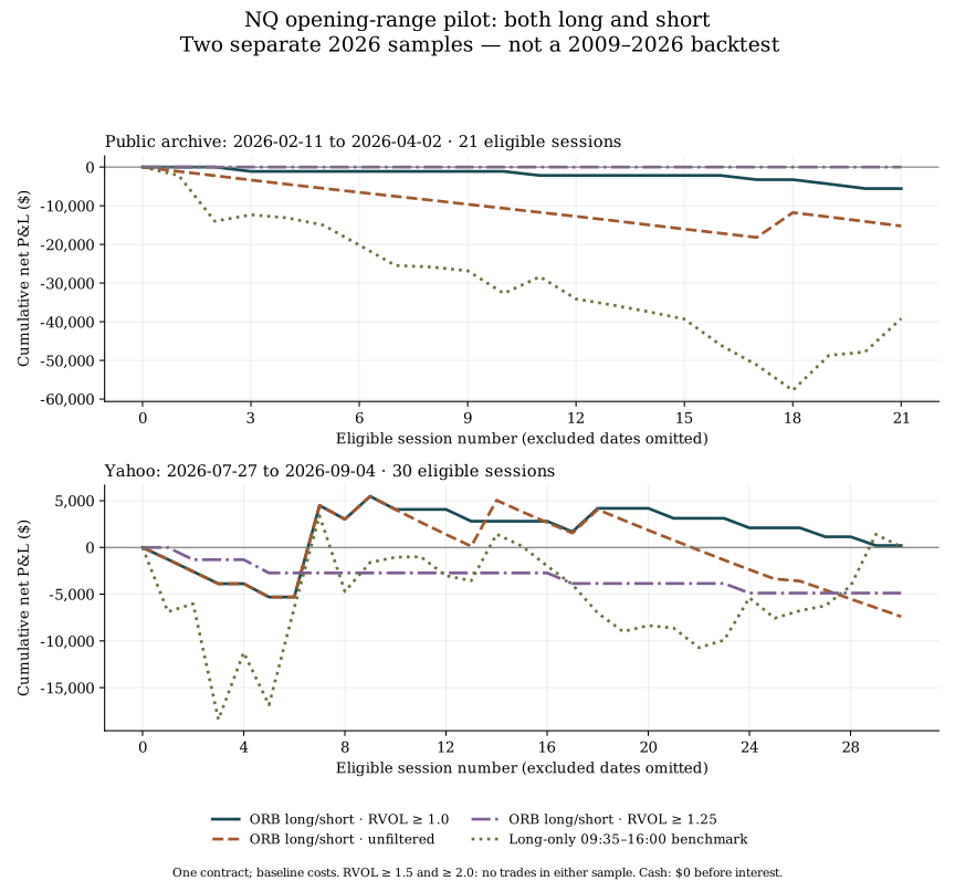
Figure 9. one NQ contract, no compounding, baseline costs. Each panel begins at zero; its horizontal axis counts eligible sessions and omits excluded dates. Vertical scales differ. Zero-trade thresholds are retained in the tables rather than interpreted as successful strategies.
Pilot assumptions and deviations
The main rule remains RVOL at least 1.0; 1.25, 1.5, and 2.0 are fixed sensitivity comparisons. Unfiltered ORB isolates the effect of the volume gate. The additional benchmark buys at 09:35 and exits at 16:00 on every eligible date, without a stop. It has different exposure and risk, so its comparison is descriptive. Cash earns zero in this accounting; interest is not modeled.
Every simulation uses one NQ contract at $20 per point and a 0.25-point tick, with $5 assumed round-trip fees. Baseline adverse fill allowance is one tick on entry and a closing exit, combining assumed spread and market slippage; protective-stop exits incur two ticks. Stress doubles those tick allowances. Neither scenario is a broker quote or a measurement of historical spreads. No percentage account returns or CAGR are reported because starting capital, margin history, and financing were not specified.
The long/short entries, outward-rounded 10%-of-ATR stop from actual fill, one-trade-per-day limit, and 16:00 exit follow the stated baseline. Gap-through fills use the worse opening price plus allowance. Intrabar entry/stop ambiguity receives the adverse feasible ordering. Fill timestamps identify five-minute bars, not observed order executions. This is not a trailing-stop test.
The files lack individual-expiry identifiers and the competing contracts needed to select by prior-session volume. RVOL therefore uses the supplied series; rollover migration cannot be verified or corrected. No quote, depth, or open-interest data were available. Full-session ATR is also approximate: a completed 18:00–17:00 ET session may supply it when at least 98% of expected five-minute bars exist. Missing bars can conceal extrema. Lower coverage resets ATR warm-up. Trading requires every bar from 09:30 through the 16:00 open; incomplete or shortened windows are excluded. The input audit and this completeness convention were recorded before ORB results.
The first usable ATR requires 14 prior true ranges after a previous close, and RVOL requires 14 prior opening intervals. These requirements and missing-data exclusions substantially reduce both samples. Excluding dates on completeness grounds can itself bias a historical sample. This exploratory replay is not an untouched out-of-sample test.
Public archive: 2026-02-11–2026-04-02
21 eligible sessions after warm-up and exclusions. ORB rows take both long and short signals. Drawdown is measured at session-end realized equity, including the initial zero balance; intraday drawdown can be larger.
| Rule | Trades | Net P&L | Net/trade | Win rate | Profit factor | EOD drawdown |
|---|---|---|---|---|---|---|
| ORB, no RVOL gate | 21 | −$15,240 | −$726 | 4.8% | 0.30 | $18,190 |
| ORB, RVOL ≥ 1.0 | 5 | −$5,555 | −$1,111 | 0.0% | 0.00 | $5,555 |
| ORB, RVOL ≥ 1.25 | 0 | $0 | , | , | , | $0 |
| ORB, RVOL ≥ 1.5 | 0 | $0 | , | , | , | $0 |
| ORB, RVOL ≥ 2.0 | 0 | $0 | , | , | , | $0 |
| Long-only benchmark | 21 | −$39,170 | −$1,865 | 23.8% | 0.39 | $57,730 |
Primary-rule P&L under doubled adverse fill allowances: −$5,605. Its baseline contains 3 flagged same-bar entry/stop cases. The approximate 95% moving-block bootstrap interval for mean net profit per trade is −$1,141 to −$1,050. With only 5 trades, this interval is fragile and does not measure uncertainty from missing data, rollover, or execution assumptions.
| Primary ORB direction | Trades | Net P&L | Net/trade |
|---|---|---|---|
| Long | 2 | −$2,295 | −$1,148 |
| Short | 3 | −$3,260 | −$1,087 |
Yahoo: 2026-07-27–2026-09-04
30 eligible sessions after warm-up and exclusions. ORB rows take both long and short signals. Drawdown is measured at session-end realized equity, including the initial zero balance; intraday drawdown can be larger.
| Rule | Trades | Net P&L | Net/trade | Win rate | Profit factor | EOD drawdown |
|---|---|---|---|---|---|---|
| ORB, no RVOL gate | 28 | −$7,395 | −$264 | 14.3% | 0.73 | $12,870 |
| ORB, RVOL ≥ 1.0 | 15 | $205 | $14 | 20.0% | 1.01 | $5,305 |
| ORB, RVOL ≥ 1.25 | 4 | −$4,880 | −$1,220 | 0.0% | 0.00 | $4,880 |
| ORB, RVOL ≥ 1.5 | 0 | $0 | , | , | , | $0 |
| ORB, RVOL ≥ 2.0 | 0 | $0 | , | , | , | $0 |
| Long-only benchmark | 30 | $80 | $3 | 50.0% | 1.00 | $18,415 |
Primary-rule P&L under doubled adverse fill allowances: $55. Its baseline contains 9 flagged same-bar entry/stop cases. The approximate 95% moving-block bootstrap interval for mean net profit per trade is −$1,151 to $1,323. With only 15 trades, this interval is fragile and does not measure uncertainty from missing data, rollover, or execution assumptions.
| Primary ORB direction | Trades | Net P&L | Net/trade |
|---|---|---|---|
| Long | 7 | $5,710 | $816 |
| Short | 8 | −$5,505 | −$688 |
Interpretation and the longer study
The baseline does not establish positive expected value: the earlier window loses money, while the later window has a small positive net result that becomes smaller under cost stress. Higher thresholds often generate no trades. A zero-trade result is absence of evidence, not proof of safety or superiority. No threshold or direction is promoted after seeing these outcomes.
The stock table’s 1,637% is its authors’ cumulative selected-stock portfolio result over 2016–2023. A compounded portfolio return and this pilot’s fixed-contract dollar P&L measure different things; neither can substitute for the other.
The chart cannot be extended backward by filling missing years or borrowing the published stock portfolio returns. The source search identified paid individual-contract NQ history beginning in late 2008, which could support a 2009 start after file-level checks. A future full study must acquire overlapping expiries, preserve the frozen rules, and evaluate rollover and execution with the required data. Its 2026 endpoint must be the latest complete available session, not the unobserved remainder of the year. See FirstRate NQ coverage.
Data provenance. The earlier file is a public TopstepX-derived archive, stored as archive.csv; the later file is a saved Yahoo NQ chart response, stored as yahoo.json. Downloads were retained before this experiment. Neither source is independently exchange-certified here. Source hashes, input audits, every simulated trade, all cost comparisons, the frozen pilot protocol, and the implementation are included in the research companion. Raw market files are kept locally and are not redistributed.
Reproduction. Run python3 books/research/orb_lab.py --input-dir PATH_TO_SAVED_FILES, then python3 books/research/orb_report.py with Matplotlib installed. The report uses a fixed seed of 42 and 3,000 circular moving-block resamples of five eligible sessions for its descriptive intervals. Excluded calendar gaps are compressed in that procedure, another limitation. Run python3 -m unittest discover -s tests -p test_orb_lab.py to verify the execution and timing invariants.
A Donchian-gated daily opening-drive
Five-minute stock ORB cannot be reconstructed on the published FAANG basket: NFLX is incomplete and GOOGL is absent. The following construction uses the archived SPY daily series instead. It is an opening-drive analogue, not a 5-minute opening-range study, not Zarattini–Barbon–Aziz's top-20 portfolio, and not the Turtle system. The protocol was frozen before the full-sample calculation.
The rule is long-only and never holds overnight. Yesterday's Channel 55/20 state, identical to the laboratory, gates today's trade. The trigger is today's open plus 10% of prior ATR(14). Survivors exit at the close. The stop is 10% of that ATR below the fill. Because the trigger sits that same distance above the open, the stop equals the open. A daily bar that both reaches the trigger and prints at or below the open does not reveal which happened first (D1). The test assumes the stop. Sessions whose planned stop cannot cover a 5 bp round-trip are skipped.
The declared edge required the gated rule to beat both the ungated opening-drive and overnight Channel 55/20 on full-sample CAGR after 5 bp costs, with neither 95% block-bootstrap interval for the mean daily-return difference lying entirely below zero. The gate failed. The combination lost less than the ungated drive and lost to the overnight channel.
Full sample, 1994-02-01–2026-07-31, 5 bp one-way:
| Rule | CAGR | Volatility | Max drawdown | Session participation | Trades |
|---|---|---|---|---|---|
| Buy and hold | 10.74% | 18.78% | −55.19% | 100.0% | 1 |
| Cash proxy | 2.46% | 0.13% | 0.00% | 0.0% | 0 |
| Channel 55/20 overnight | 3.59% | 9.16% | −29.45% | 48.9% | 160 |
| Opening-drive, ungated | −30.50% | 2.43% | −100.00% | 55.9% | 4,569 |
| Opening-drive, Donchian-gated | −8.47% | 1.54% | −94.84% | 18.3% | 1,496 |
| Opening-drive, gated, no economic skip | −17.64% | 1.76% | −99.82% | 41.4% | 3,385 |
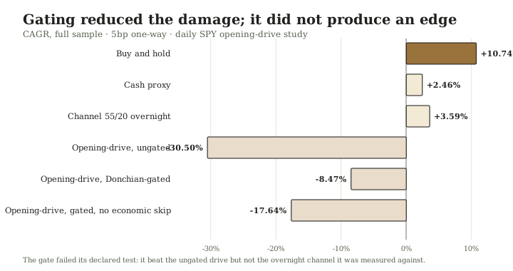
Figure 10. the same six rows as the table above. Gating cut the ungated drive's loss by more than half; it still did not reach the overnight channel it was measured against.
Of 1,496 primary fills, 1,494 are flagged same-bar stops. Annualized mean daily-return differences versus buy-and-hold and versus Channel 55/20 have 95% intervals entirely below zero (−26.56% to −14.82%, and −16.37% to −9.36%). The interval versus the ungated drive is entirely above zero: the gate reduced damage by trading less often. At 25 bp the economic skip produces no gated trades, so the primary rule earns the cash proxy. Chronological slices and the 25 bp table are retained in the companion.
Research conclusion. Combining these two tools on daily bars did not produce an edge against the simpler overnight channel. The adverse same-bar convention is doing most of the work: a daily OHLC series cannot certify that an opening drive held. That is a data limitation, not a license to assume the favorable order or to retune the stop after seeing the loss. A later 5-minute reconstruction would need a completed opening-range high, not this open-plus-offset analogue. The inference chapter treats this as a convention loser: the opposite fill is equally unsupported, and computing it after the loss would manufacture a winner the bar does not contain.
Reproduction. Read books/research/expansion/SPINOZAN-ORB-PROTOCOL.md, run python3 -m unittest discover -s tests -p test_orb_donchian.py, then python3 books/research/orb_donchian.py. Outputs are orb-donchian-results.json and ORB-DONCHIAN-RESULTS.md. The calculation uses the same archived SPY and French RF inputs as the indicator laboratory.
Chapter 41
The Turtle Traders
In 1983 Richard Dennis wagered that trading could be taught. William Eckhardt wagered that it could not. They advertised for apprentices, trained a class, and gave them real futures accounts. Curtis Faith, one of those apprentices, later published the rules they were taught. Two claims in that record must be kept apart. One is a philosophy: a complete mechanical system plus the discipline to follow it. The other is a performance story: Faith reports that the group compounded at about 80% a year during the experiment. This edition uses the published rules. It did not audit the original ledgers. Faith 2003.
The philosophy is more durable than any one year's return. Faith quotes Dennis, via Schwager, that the rules could be printed in a newspaper and still not be followed. The binding constraint is consistency through losing streaks, not secrecy. A complete Turtle system specified markets, volatility units, entries, stops, exits, and order tactics. An incomplete copy that keeps only “buy the 20-day high” is a different method.
What they actually traded
N is a 20-day ATR. Faith seeds it with a 20-day simple average of true range and then updates Nₜ = (19 Nₜ₋₁ + TRₜ)/20. A Unit is the integer number of contracts such that one N of price movement equals one percent of the notional account:
Unit = floor(0.01 × Equity / (N × dollars per point)).
Stops sat 2N from the fill, so one unit that exits at the trigger loses two percent of equity, not one. Additional units were added every ½N from the prior fill, and earlier stops were raised by ½N so that the stack's planned stop generally sat 2N from the newest unit. Single-market exposure was capped at four units; closely correlated markets at six; loosely correlated markets at ten; one direction of the whole book at twelve. After a 10% loss from the working notional, they cut that notional by 20% and resized.
System 1 entered one tick beyond the prior 20-day high or low and exited on a 10-day opposite breakout. A System 1 entry was skipped if the previous breakout in that market would have been a winner, with a 55-day failsafe so a major move was not missed. System 2 entered on a 55-day breakout, took every signal, and exited on a 20-day opposite breakout. Traders could allocate equity between the two systems.
These are futures rules. Contract multipliers, rolls, daily limits, and opening gaps are part of the method. A stock or ETF close-confirmed channel is not a substitute.
Proposition TT1If one N equals fraction f of equity, a 2N stop that fills at the trigger loses 2f of equity.
Assumptions. Equity is V>0. One unit has quantity q such that q N M = f V, where M is the dollar value of one price point. The stop fills at a price exactly 2N adverse to the entry.
Demonstration. The dollar loss is q·(2N)·M = 2f V. The fractional loss is 2f. ∎
Faith's unit uses f=0.01, so a clean 2N exit costs 2% of the working account. The identity does not bound a gap through the stop.
Proposition TT2A four-unit stack filled at exact ½N intervals, with every stop set 2N below the newest fill, has planned stop-distance loss 5f of equity.
Assumptions. A long stack is filled at p, p+½N, p+N, and p+1½N. After the last add, every unit's stop is 2N below the newest fill. Each unit satisfies q N M = f V, and the common stop fills at its trigger.
Demonstration. Write the newest fill as p*. Remaining adverse distances are 2N, 1½N, N, and ½N. The corresponding dollar losses are 2f V, 1.5f V, f V, and 0.5f V. Their sum is 5f V. ∎
A common retelling says the whole loaded market risks 2%. That is the Whipsaw alternate, which used ½N stops and therefore four units × ½f = 2f. The standard 2N stack with lifted stops is larger. Planned heat is still not a maximum realized loss.
Proposition TT3Skipping a 20-day breakout after a winning prior breakout produces a different entry set from taking every 20-day breakout.
Construction. Market A has a winning 20-day breakout, then another 20-day breakout before any 55-day failsafe. System 1 skips the second entry. A take-every-20-day rule takes it. The two event sets differ. ∎
The skip rule is a different strategy, not a cosmetic filter. Faith counts the prior breakout as a winner or loser even if it was itself skipped. A test that omits that bookkeeping is not System 1.
Proposition TT4A unit-count cap does not bound loss when the fill can gap through the 2N stop or N is stale.
Construction. Four long units have a common stop 2N below the newest fill. The next session opens 6N below that fill with no trade at the stop. If market orders are elected, the realized loss is about 6f V per unit, or 24f V for the stack, not the planned 5f V of TT2. Separately, if N was computed last week and true range has doubled, the same contract count now represents twice the intended dollar volatility. ∎
Faith records that the day after the October 1987 crash produced losses of 20% to 40% of equity in interest-rate futures despite the unit caps. The caps reduced what the loss would otherwise have been. They did not make it small.
Proposition TT5A long-only close-confirmed channel on one equity index is not the Turtle System.
Construction. The Turtle book is long and short many futures, sized in N-units, pyramided, stop-limited, and correlation-capped. A rule that buys one stock-index ETF when its close exceeds a 55-day high and holds cash after a 20-day low has a different universe, direction set, size, execution, and risk. The two objects are not identical. ∎
This edition's laboratory Channel 55/20 is the second object. From 1994 through July 2026, at 5 bp one-way, it compounded at 3.59% with a −29.45% drawdown and spent about half the sample in cash. Its paired intervals versus buy-and-hold lie below zero under the laboratory's approximation. That is evidence about a modern single-index cousin. It is not a Turtle reconstruction, and it does not show that the Turtle book failed.
Proposition TT6A historical multi-asset trend premium does not entail that every Donchian parameterization is profitable after costs.
Construction. Suppose a diversified 1-/3-/12-month futures combination has positive mean excess return in a stated sample. A 20-day breakout on one market, or the same combination after doubled costs and a skipped-winner filter, is a different payoff. The first mean does not determine the sign of the second. ∎
What later public evidence can show about modern markets
The Turtle experiment ended decades ago. Modern viability is a different empirical question. Two public research programs study diversified trend following, not Faith's exact unit book.
Hurst, Ooi, and Pedersen construct a hypothetical equal-weighted mix of 1-, 3-, and 12-month time-series momentum on up to 67 markets from 1880 through 2013. In their full sample, after stated costs and fees, they report about 11.2% annualized return, 9.7% volatility, and a Sharpe ratio of 0.77, with near-zero correlation to U.S. equities. The strategy's annual returns form a “smile” against extreme equity years, and they record positive returns in 8 of the 10 largest 60/40 drawdowns. They also note post-2008 correlation spikes and hypothetical-data limits. AQR paper.
Lempérière, Deremble, Seager, Potters, and Bouchaud extend trend tests across four asset classes over two centuries. They report excess-return t-statistics of about 5 since 1960 and about 10 since 1800 after removing long-only drift. Long-horizon trends show no statistical degradation in their recent window; trends of a few days have withered since about 1990. Author paper.
Huang, Li, Wang, and Zhou, using the original Moskowitz–Ooi–Pedersen futures set, find little asset-by-asset twelve-month predictability and a pooled t-statistic that fails their bootstrap. A time-series-momentum book can still make money while looking like a historical-mean book. That weakens a naive sign rule. It does not erase every multi-horizon, multi-asset construction. Journal of Financial Economics paper.
Taken together, the public record supports a narrow modern claim: diversified, volatility-scaled trend following has a long historical sample, including late-twentieth-century and early-twenty-first-century windows, in which researched portfolios were profitable before or after the authors' cost models. The same record does not support the claim that a 20-day breakout on a single modern equity index, or an unaudited copy of 1980s contract lists, inherits that result. This edition did not reconstruct the Turtle futures book.
Usefulness verdict
The Turtle philosophy is a complete-system doctrine: define the bet, size it in current volatility, cap correlated heat, cut the working stake after losses, and do not abandon the rule because a streak is unpleasant. Those are risk and process claims. The geometric identities above make the unit arithmetic inspectable. The modern literature makes a diversified trend family historically serious. Neither is a proof that the next 20-day breakout is a good trade.
A reader who wants to research the family should write a futures protocol: eligible contracts, rolls, N convention, unit equity, skip-rule bookkeeping, correlation groups, and a cost model. Compare it with a passive risk-matched allocation and with the simpler monthly filter already tested here. Reject any transfer of Faith's 80% figure, or of Hurst's 1880–2013 Sharpe ratio, onto an untested account.
Sources. Faith 2003; Hurst, Ooi and Pedersen; Lempérière and coauthors; Huang, Li, Wang and Zhou; this edition's Channel 55/20 laboratory. TT1–TT6 are original demonstrations. The risk-management chapter treats heat, gaps, and the 10/20 reduction rule as general tools.
Chapter 42
Risk Management
Risk management is the part of a strategy that remains after the forecast is written down. It decides how large a bet may be, what happens when the bet is wrong, which losses are allowed to occur together, and when the operator must stop. It does not create a positive expected return from a fair or losing game. Proposition 18 already forbids that substitution. The usefulness of these tools is survival, comparability, and the prevention of a single error from ending the experiment.
A complete risk plan names more than a stop. Market risk is the ordinary movement of prices. Gap and limit risk is movement that skips the planned exit. Liquidity risk is the inability to exit at a meaningful size. Correlation risk is the failure of “many names” to be many bets. Financing and margin risk can close a position before its thesis matures. Model risk is a mis-measured N, beta, or volatility. Operational risk is a wrong clock, a missed roll, or a frozen worksheet. These are different objects. A single percentage cannot represent all of them.
A risk worksheet
Complete this beside the strategy worksheet. If a cell is empty, the account is improvising.
| Field | What to write |
|---|---|
| Risk unit R | The dollar loss assumed if the planned exit fills at its trigger |
| Heat | Open planned loss if every current stop fills at its trigger |
| Hard cap | Maximum R, heat, gross leverage, and per-market contracts |
| Correlation groups | Which positions count as one bet, and the group cap |
| Gap rule | What happens if the next print is through the stop |
| Resize rule | How equity, N, or volatility updates quantity, and how often |
| Loss-cut rule | When working capital is reduced after a drawdown |
| Pause rule | Operational faults that forbid new risk |
| Ruin / withdrawal | Capital that must not be used, and the drawdown that ends the method |
One risk unit is not a guaranteed maximum loss. Heat is not realized drawdown. A pause rule is not a prediction that history will respect it.
Proposition RM1Cutting working equity by fraction α after a drawdown replaces subsequent unit size by the factor 1−α.
Assumptions. Unit quantity is proportional to working equity V, with N and dollars-per-point held fixed. After the cut, the operator uses (1−α)V.
Demonstration. The unit formula is q = floor(c V / (N M)) for a stated constant c. Replacing V by (1−α)V multiplies the unrounded size by 1−α. ∎
The Turtles cut notional by 20% after a 10% loss from the working account, then again if another 10% of the reduced account was lost. That is a survival rule. It also reduces participation in the next favorable run. A trader who cuts only after a loss and never restores size except at a yearly reset has chosen a path-dependent exposure. Record the restore rule; do not leave it to mood.
Proposition RM2Under a linear return model, multiplying every holding by k multiplies expected P&L by k and variance by k².
Assumptions. Portfolio P&L is Σ qᵢ Xᵢ with finite second moments. Replace each qᵢ by k qᵢ.
Demonstration. E[Σ (k qᵢ) Xᵢ] = k E[Σ qᵢ Xᵢ]. Variance scales by k² because Var(kY)=k² Var(Y). ∎
Halving size halves expected profit and quarters variance in this model. It does not turn a negative-mean process positive. It does change the chance of hitting an operational ruin threshold before a long-run mean, if that mean exists, can be expressed. Sizing is therefore part of the strategy, not a later decoration.
Proposition RM3A volatility target does not imply a bound on maximum drawdown.
Construction. Let each period's return be ±σ with equal probability, independently, after an exact volatility target has set |wσ|=σ. After n periods the wealth factor is a product of n terms (1±σ). The path of n consecutive losses has probability 2⁻ⁿ>0 and drawdown 1−(1−σ)ⁿ, which exceeds any fixed multiple of σ* once n is large enough. ∎
Proposition P2 showed that an exact conditional volatility estimate can set next-interval volatility. That is a one-step identity. Drawdown is a path functional. A 10% volatility target is compatible with a 40% decline. Value-at-Risk and expected shortfall are similarly one-horizon statistics under a stated law. They are useful only beside stress paths that the law may omit.
Proposition RM4A correlation cap computed from past returns can fail as a loss cap when those correlations rise to one.
Construction. Two unit-sized positions were treated as loosely correlated and therefore allowed together under a ten-unit group cap. On the shock day their returns are identical. Portfolio variance that day is the variance of a single doubled position, not the historical two-asset formula. The planned diversification term (1−ρ) vanishes. ∎
Turtle group caps, risk-parity weights, and “twelve uncorrelated systems” all depend on a relationship estimated from calmer data. Faith's 1987 interest-rate example is the operational form of this proposition: several permitted units became one bet overnight. A stress sheet that sets ρ=1 inside each declared group is a more honest heat number than the average pairwise correlation of the last year.
Proposition RM5Planned heat is not realized drawdown.
Construction. Heat is defined as the sum of planned trigger losses on open positions. A position with heat 2% gaps to an 8% loss. Realized drawdown includes that 8% and also closed-trade losses that are no longer in heat. Conversely, an account can show large heat while prices have moved in its favor and no drawdown has been printed. The two numbers answer different questions. ∎
Report both. Heat answers “what we have chosen to lose if exits fill as written.” Drawdown answers “what the equity curve has already lost.” Gap, liquidation, and finance costs live in a third column: unplanned loss.
Proposition RM6No finite catalog of stops, sizes, and diversification rules identifies a favorable future under unrestricted distribution change.
Construction. Two markets agree on every observation through date T, including every fill that the risk rules used. After T, one continues to pay the planned 2N exits; the other gaps by ten times N whenever a stop is due. Any rule written from the first T observations issues the same orders in both worlds. The history does not identify which continuation occurs. ∎
This is the risk-management form of Proposition S4. Learning is still possible under restricted change: stable contract mechanics, slowly moving volatility, or a declared stress that the account must survive even if the forecast is right. The result is an argument for writing those restrictions down, not an argument for having no risk plan.
Rules that survive contact with the account
A defensible plan uses several independent brakes rather than one clever threshold.
Size from current risk, not from conviction. ATR or variance units compare markets. Conviction is not a unit of account.
Cap the bet, the group, and the book. Per-market, correlated-group, and directional caps are different. Write all three.
Assume the stop can miss. A gap rule either reduces size, uses options, or accepts that a day like Faith's 1987 example can occur.
Reduce after loss by a written schedule. The Turtle 10/20 rule is one schedule. A volatility target that shrinks when realized variance jumps is another. Changing the schedule after a loss is a new strategy.
Keep non-risk capital out. Money needed for near-term obligations is not working equity. A method that requires the rent in order to recover is already in default.
Pause for operations, not for boredom. Missing data, a broken clock, an untradeable roll, or an account that no longer matches the worksheet are pause events. A dull month is not.
The monthly filter, the daily laboratory, and the Turtle unit book each need this sheet filled with their own numbers. Copying another trader's 2% stop into a different clock or instrument changes the object.
Usefulness verdict
Risk management is useful when it makes the intended loss explicit, keeps correlated bets from silently adding, and leaves enough capital to execute the next valid signal. Its identities can be proved. Its parameters cannot be deduced from Euclid. The Turtle rules are a historically complete example of such a plan. They are not a proof that 2N, four units, or a 20% notional cut is optimal.
Evaluate a risk plan by the losses it was designed to survive and by the opportunities it refuses. A plan that never permits a 20% decline may also never permit the trend that pays for the failed breakouts. State that tradeoff. Then keep the ledger honest when the gap arrives.
Sources. Faith 2003 on units, caps, and the 10/20 cut; Propositions 11–20 and P1–P3; Hurst, Ooi and Pedersen on trend-following drawdowns. RM1–RM6 are original demonstrations in this edition.
Chapter 43
Where a Trading Edge Can Come From
An indicator is a function of a history. A strategy is a rule that turns a history into holdings. An edge is a favorable comparison of that rule against a stated alternative, after costs, under a probability law that has not been granted by the formula. The three objects are routinely collapsed into one sentence: “the crossover has an edge.” That sentence names a recoding and asserts a payment. It does not identify who pays, or why.
This chapter separates sources that can, in principle, transfer money from sources that only rename the same tape. It does not prove that any listed source is currently available to a retail account. It does prove that several popular claims are not sources at all.
Six families, not a fifth source in the chart
The following families are distinct enough to keep apart. They can overlap in a working business. They are not interchangeable labels.
Risk transfer. Someone wants to shed a risk others will hold for a price. Insurance, some futures hedges, and some option-selling books live here. The payer is identifiable in the story: a hedger, a constrained institution, or a holder who values certainty more than the seller values the premium. A risk premium can exist without a chart pattern. It can also fail to cover the seller’s tail.
Inventory and spread. A dealer or maker is paid to hold what others wish to trade now. The visible spread is one term; fill-conditioned markout, inventory, and fees are the others. Propositions L1–L3 already show why a posted spread is not a coupon.
Speed and queue. A participant who arrives first, or who occupies a better queue slot, can capture a discrepancy that is gone before a slower order is eligible. The clock includes infrastructure, not the timestamp printed later. A public snapshot of an opportunity is not evidence that the observer could have been first.
Information that is not in the chart. A forecast that uses observations absent from H, the price-and-volume history already on the screen, can, in principle, change the conditional distribution of the next tradable increment. Corporate events, order-book data the chart never saw, and privileged inventory knowledge belong here when they are actually available before the order. Another moving average computed from the same closes does not.
Forced flow. A participant must trade for a reason other than the conditional mean: a redemption, a roll, a rebalance, a margin call, an index addition. The other side is paid, if at all, for absorbing that urgency. The existence of forced flow is not a fill at a favorable price.
Rule-set optionality. A fee paid for a right whose loss is bounded by that fee is a contract about a constrained game, not a proof about the underlying’s expectancy. Evaluation accounts, challenges, and some prize structures live here. EG3 and the prop-firm chapter treat the geometry.
Indicators, candles, and named crossovers are recodings of H. They can be useful as compressions, risk states, or execution triggers. They are not a seventh family and not a fifth source hiding inside the first four. U1 already forbids an ideal decision maker from gaining information by restricting itself to a function of H. The next proposition records the corresponding fact about source.
Proposition EG1An indicator computed from H is not a source of edge distinct from H.
Assumptions. H is the information available at the decision. I = f(H) for a deterministic function f. An edge is a favorable comparison of expected objective, after the same costs, against a stated alternative, under a common probability law.
Demonstration. Every action that is a function of I is a function of H. Therefore any expected-objective comparison available from I is already available from H. I cannot be a source of expected advantage that H does not contain. ∎
Scholium. This does not say that a compression is useless. A finite trader can execute a two-state filter more consistently than a thousand raw prints. Usefulness of that kind is operational. It is not a new payer. Ten recodings of the same closes remain one history.
Proposition EG2Two strategies that induce the same predictable holdings have the same expected gain under the premises of U3.
Assumptions. The premises of U3 hold. Strategies A and B choose bounded predictable positions q^A and q^B from H. On the relevant horizon, q^A_t = q^B_t almost surely for every t.
Demonstration. Gross discounted gain is G = Σ q_t (S_{t+1} − S_t). Identical positions give G^A = G^B, hence E[G^A] = E[G^B]. Under U3 that common value is zero before costs. ∎
Scholium. A MACD cross and an EMA-ordering rule that produce the same long-or-cash sequence are one book with two names. Changing the picture does not change the holdings. Changing the holdings can change the gain; that is a different experiment. Costs that depend on how the state was computed, rather than on the positions traded, must be stated separately. Under the laboratory’s next-open convention they are not.
The random-rule study in the laboratory results keeps this distinction operational. Destroying the dates of a channel’s long days, while preserving how many long days occurred, is a change of holdings. An iid coin-flip is another change of holdings. Neither control is a new source of edge. Both are allowed to beat the named rules. On this edition’s tape they did not beat buy-and-hold, and the coin-flip’s 95% interval versus the EMA50/200 book lay entirely below zero.
Proposition EG3A fee paid for a right whose loss is bounded by that fee is not a proof about the underlying’s expectancy.
Assumptions. A buyer pays a nonrefundable fee F > 0 for a right whose subsequent cash outcome Y satisfies Y ≥ −F. The underlying account, if traded with the buyer’s own capital and without that contractual floor, has payoff X.
Demonstration. Y is a different random variable from X. The inequality Y ≥ −F can hold whether E[X] is positive, zero, or negative. Observing that someone paid F, or that a particular realization of Y was positive, does not determine the sign of E[X]. ∎
Worked case. A challenge fee buys a path-dependent evaluation with a stated profit target and a stated knockout. Completing the evaluation is a fact about that constrained path. It is not a measurement of the instrument’s expected excess return, and it is not a withdrawable payout under a later account’s rules. The prop-firm chapter supplies the geometry and the dated official pages.
What this edition has and has not shown
The comparative laboratory and the monthly filter are statements about specified SPY/cash rules against buy-and-hold and cash. They are not a census of risk premia, dealer businesses, or speed advantages. The opening-drive analogue failed its declared edge gate. The Turtle chapter specifies a futures system and cites later trend papers; it does not reconstruct a personal book.
Public research already in the inference chapter, Sullivan–Timmermann–White, McLean–Pontiff, Novy-Marx–Velikov, Hou–Xue–Zhang, Huang and coauthors on time-series momentum, concerns searched families, post-publication decay, costs, and reconstruction. Those papers are the honest neighborhood of “simple rules versus elaborate ones.” They are not a single theorem that coin flips beat every complex strategy.
A trader who cannot name which of the six families could pay the account has not specified an edge. Naming a family is still only a hypothesis. The strategy worksheet is where that hypothesis becomes a test. Calling the hypothesis “Renaissance” does not supply a family; the algorithmic-trading section is the institutional counterexample.
Usefulness verdict
The universal claim that “the chart contains the edge” fails: a recoding of H is not a distinct payer. The universal claim that “indicators never help” also fails: measurement, sizing, and consistent execution can be useful without being sources. The remaining work is empirical and institutional. It is not solved by adding another oscillator.
Source notes
Usefulness identities U1–U3 and liquidity identities L1–L3 are original to this edition. The random-rule protocol is books/research/expansion/RANDOM-PROTOCOL.md. Official evaluation pages used for EG3’s institutional examples are listed in books/research/expansion/prop-firm-sources.md. No live edge is claimed.
Chapter 44
Prop Firms and Challenges
A prop-firm challenge is a purchased evaluation. The buyer pays a fee for a simulated account that must hit a profit target without violating stated loss and consistency rules. Passing that evaluation is a path event. It is not a proof that the underlying instrument has positive expectancy, and it is not a withdrawable payout. Those are three different objects. Treating them as one sentence, “I passed, so I have an edge, so I have income”, is the error this chapter removes.
The rules below are dated to the official pages inspected in September 2026. Firms rewrite parameters. Recheck the current help pages before sitting an evaluation. This edition does not estimate how often traders pass, how often they are paid, or whether any firm’s contract is a good purchase. Those frequencies are not in the official pages used here, and blog percentages are not book-grade evidence.
Three objects that share a dashboard
The evaluation. A finite, rule-constrained knockout. Typical pieces are a profit target, a maximum loss, sometimes a daily-loss halt or fail, a consistency or best-day cap, a minimum number of days, and a contract-size cap. Topstep’s Trading Combine is described as a simulated account with one rule, do not let the balance hit or go below the Maximum Loss Limit, and two objectives: reach and maintain the profit target, and keep the best day below 55% of that target or the target rises. FTMO’s 1-Step Challenge uses a 10% profit target, a 3% daily-loss limit recalculated at midnight CE(S)T, a 10% end-of-day trailing maximum loss, and a Best Day Rule of 50% of Positive Days’ Profit. FTMO’s 2-Step Challenge uses 10% then 5% targets, a 5% daily loss, a 10% static maximum loss, and at least four days on which a position is opened. Topstep Combine parameters; FTMO trading objectives.
The underlying game. The instrument’s expected P&L if the same trades were done with the trader’s own capital and without the evaluation’s floor. That expectancy is what EG3 says the fee does not prove.
The payout. A later contractual transfer, if any, under a later account’s rules. Topstep states that Combine profits do not carry into the Express Funded Account. FTMO states that all accounts it provides are demo accounts with fictitious funds, and that the subsequent FTMO Account has no profit target. A screenshot of a passed Combine is not a bank credit.
A zero-edge grind can pass. A positive-expectancy trend book with Turtle-sized heat can fail a daily-loss or trailing-drawdown rule. Both facts follow from the geometry, not from a trader’s character.
Proposition PF1A profit-target and daily-loss evaluation can accept a zero-mean path and reject a positive-mean path.
Construction. Start at 100. The evaluation accepts a closed-equity path if some close is at least 110 and no close is 5 or more below that day’s starting wealth; otherwise it rejects.
Path A: 104, 108, 110. Daily changes +4, +4, +2. No daily loss of 5. Accepted. The path is a permitted realization of a symmetric random walk, a canonical zero-mean process.
Path B: 120, 114. Daily changes +20, −6. The average increment is positive. Day 2 starts at 120 and ends at 114, a daily loss of 6. Rejected. ∎
The evaluation is a pair of barriers plus a target. It is not a test of the generating mean. Optional daily-loss halts that flatten the book without failing the account, Topstep’s optional Daily Loss Limit, which the help center says is a session break and not a Combine fail, change the path without converting the evaluation into an expectancy estimator. Daily Loss Limit.
Proposition PF2Completing an evaluation does not entail positive expectancy after the evaluation.
Assumptions. Before the evaluation ends, positions are bounded and predictable. After it ends, the trader faces either the same instrument without the evaluation’s contractual floor, or a new account whose rules are a different contract. Expectancy is E[X] for the post-evaluation payoff X.
Demonstration. Completing the evaluation is the event that a constrained path hit its target without a knockout. That event is a function of the evaluation path. It does not appear among the premises that determine E[X] on the later filtration. In particular, if post-evaluation increments remain a martingale increment sequence under the premises of U3, then E[X] = 0 before costs regardless of the evaluation’s outcome. If the later contract changes the sharing rule, the reset, or the trailing loss, X is a different random variable again. ∎
Scholium. A pass can be followed by a payout, a later fail, or a reset. None of those observations retroactively estimates the instrument’s mean. Faith’s Turtle heat identities in the Turtle chapter already show why a book sized for a 20–30% account swing is a poor match for a 3–5% daily barrier. The mismatch is geometric.
Proposition PF3A rule that limits the fraction of profit on one day excludes some positive-expectancy policies that concentrate gains.
Construction. Start at 100. A policy is eligible only if its single best day is at most half of its total closed profit. Policy C earns +20 on day 1 and 0 thereafter. Its best day is 100% of total profit, so it is ineligible. Policy D earns +2 on each of ten days. Its best day is 10% of total profit, so it is eligible. Let the instrument’s remaining increments after day 1 be independent of C’s first-day gain, with nonnegative conditional expectation. Then C can have E[total profit] > 0 while remaining ineligible. ∎
Institutional examples, not additional proofs. Topstep’s Combine requires the best day to stay at or below 55% of the profit target (equivalently, Best Day ÷ 0.55 is the total needed if the best day overshoots). Losses do not reset the best day. FTMO’s 1-Step Best Day Rule requires the best day not to exceed 50% of Positive Days’ Profit; exceeding it is not a breach, but more profit must be earned. Topstep consistency; FTMO trading objectives.
A concentrated +EV event, the gap the Turtle book is built to hold, is exactly what these caps penalize. That is the point of the rule from the firm’s side. It is also why “I trade my live system on the challenge” can be a category error.
How to sit a challenge without confusing it for a market test
Write the knockout sheet before the first order. Copy the current official numbers; do not copy this paragraph’s dated examples as if they were still in force.
| Field | What to write from the current page |
|---|---|
| Fee and what it buys | The evaluation only, or also a later account, reset, and data |
| Profit target | Percent or dollars, and whether it must be maintained with positions closed |
| Maximum loss | Static, end-of-day trailing, or intraday; from initial capital or from a peak |
| Daily loss | Fail, optional halt, or absent; the clock that resets it |
| Consistency / best day | Numerator, denominator, and whether a breach fails or only raises the target |
| Minimum days | What counts as a trading day |
| Size cap | Contracts, micros, and whether they scale |
| What transfers | Combine or Challenge P&L, if anything |
| What “funded” means | Simulated, live, payout eligibility, and the next knockout |
Size so that a day the live method treats as ordinary noise does not touch the daily barrier or the maximum loss. If that size makes the profit target unreachable inside the trader’s actual distribution, the evaluation is a poor match for that method. The correct response is to decline the purchase or to sit a different constrained game, not to hide size, split accounts against a stated single-profile rule, or otherwise evade the contract. This book will not teach evasion.
Treat the fee as the premium for a capped-downside option on a path. EG3 already says that premium is not a measurement of the underlying. A pass is a selected path. A payout, if it occurs, is a later contract. A livelihood is a third question, answered by the operation chapter: persistent skill among Taiwan day traders was below 1% in Barber, Lee, Liu, and Odean; 97% of Brazilian equity-futures day traders with more than 300 days lost after fees in Chague, De-Losso, and Giovannetti. Those studies are not prop-firm pass rates. They are the evidence that remains when the dashboard is stripped of its marketing.
What succeeding means here
Succeeding at a challenge means meeting the written objectives and, if that is the aim, becoming eligible for whatever payout the later page describes. It does not mean the strategy has positive expectancy on the instrument. It does not mean the household has a dependable income. It does not mean the Combine’s dollar P&L is capital. Topstep’s help center states that Combine profits do not transfer. FTMO’s page states that the accounts are simulated.
A trader can succeed at the constrained game and still have no edge in the underlying game. A trader can have an edge in the underlying game and fail the constrained game. Both sentences can be true at once. The worksheet is the place to say which game is being played.
Source notes
Official pages and the decision not to use blog pass rates are recorded in books/research/expansion/prop-firm-sources.md. Geometric identities PF1–PF3 are original to this edition. Livelihood figures remain the studies already cited in the operation chapter. No personal challenge result is used.
Chapter 45
The Anatomy of a Repeatable Edge
Futures and currencies are where the public record of systematic trading is longest, widest, and most contested. Researchers have reconstructed diversified trend-following portfolios across dozens of futures markets back into the nineteenth century (later public evidence). Carry, the return from holding a higher-yielding currency or a contract priced below spot, has decades of documented premia and documented crashes. Hedgers, central banks, index rebalancers, and benchmark fixes create flows whose participants have reasons to trade other than a forecast. These are the markets where the question "who pays me, and why would they keep paying?" has the most concrete candidate answers.
This Part asks what a repeatable edge would have to be, which strategy families have public records that meet some of its conditions, and how an individual could build, test, operate, and retire one. It keeps the book's discipline. Every empirical statement names its study, sample, and cost treatment. Every proposition states its assumptions. This edition has run no forex or futures backtest of its own, so nothing in this Part is a result of the book's laboratory. Where a blueprint is untested, it says so.
What repeatable has to mean
Definition. A repeatable edge is a fully specified rule, together with a stated comparison policy, that meets five conditions.
- A named payer. The rule accesses one of the families in Where a Trading Edge Can Come From: risk transfer, inventory and spread, speed and queue, information not in the chart, forced flow, or rule-set optionality. The family explains why a counterparty accepts the expected loss.
- A net margin. Its expected return after fees, spreads, slippage, financing, and roll exceeds the comparison policy's, at the account's actual size.
- Breadth. It holds across a class of markets or occasions chosen before testing, not in one instrument selected afterward.
- Stability. It holds across time slices and neighboring parameter values, and it has survived publication or has a live record after its discovery.
- Survivability. Its drawdowns, losing periods, and tail events fit the capital and obligations of the person operating it.
Each condition can fail while the others hold. A real risk premium can be too small to pay a retail spread. A cheap, stable effect can depend on a flow that a regulator or a benchmark provider removes. A diversified, cost-efficient premium can still lose for five years, and an account that needed monthly income will have closed before the expectation expresses itself. The five conditions are a checklist, not a score to be averaged.
| Condition | The question to answer in writing | Where this Part treats it |
|---|---|---|
| Named payer | Who takes the other side, and why do they keep doing so? | Edge families and each strategy chapter's mechanism section |
| Net margin | Does the gross margin survive the speed at which the rule trades? | RE2, instruments, operation |
| Breadth | How many independent bets does the rule actually place? | RE1, CX1, portfolio construction |
| Stability | Did it survive its neighbors, its time slices, and publication? | TM1, the edge factory |
| Survivability | Can the account and the person hold through its worst plausible path? | TF2, CY3, EF3 |
Principles that recur in durable public records
Read the public records of long-lived systematic futures and currency programs, the academic literature on their families, and the histories of strategies that did not last, and a small set of principles recurs. None is a forecast. Each is either a mathematical consequence proved in this book or a regularity in the sourced evidence of the chapters that follow.
Be paid by someone with a reason to pay. A chart pattern is a recoding of the price history (EG1). A hedger shedding risk, an investor paying to avoid crash exposure, or a fund that must rebalance on a schedule is a reason. Each family with a long public record in this Part has a candidate payer. The popular methods that lack one also lack credible evidence.
Place many unrelated bets. Breadth is the one principle whose benefit follows from arithmetic alone (RE1), and correlation sets its limit. Ten tickets that are all short the dollar are one bet (CX1).
Size by risk, not by conviction. A position's size should come from the instrument's volatility and the account's risk budget (risk management). Micro contracts make that arithmetic possible in small accounts (FM3).
Match speed to cost. The same cost per trade is negligible for a slow rule and fatal for a fast one (RE2). Most of the documented premia in this Part trade slowly.
Know the shape of the payoff. A strategy with positive skew, such as diversified trend following, can lose modestly for years while its expectation is positive (TF2). A strategy with negative skew, such as carry or volatility selling, can earn smoothly for years while its expectation is negative (CY3). A trader who does not know which shape a strategy has will abandon the first at the wrong time and enlarge the second at the wrong time.
Survive first. Zero capital is absorbing (Proposition 10). No expected return is collected by an account that has closed. Leverage, gaps, margin increases, and correlated losses are the usual causes (FM4, OP1, RM4).
Keep few parameters and fix them in advance. Every free choice made after seeing results is part of a search (statistical inference). The constructions with the longest public samples in this Part can each be stated in a short paragraph.
Measure against a declared alternative and retire by rule. An edge is a comparison, so it needs a benchmark, a horizon, and a retirement rule written before the evidence arrives (the edge factory).
Proposition RE1Equal-weight combination of N return streams with common Sharpe ratio S and common pairwise correlation ρ has Sharpe ratio S√(N/(1+(N−1)ρ)).
Assumptions. Each stream has expected excess return μ and standard deviation σ > 0 over the same period, so S = μ/σ. Every pair of streams has correlation ρ, with 1+(N−1)ρ > 0. The combination holds weight 1/N in each stream.
Demonstration. The combination's expected excess return is μ. Its variance is (1/N²)(Nσ² + N(N−1)ρσ²) = σ²(1+(N−1)ρ)/N. Dividing the mean by the standard deviation gives (μ/σ)√(N/(1+(N−1)ρ)). ∎
Scholium. With ρ = 0, ten streams multiply S by √10 ≈ 3.16. With ρ = 0.2, twenty streams multiply it by about 2.04, and no number of streams can multiply it by more than 1/√0.2 ≈ 2.24, because the factor tends to 1/√ρ as N grows. Breadth has the most dependable arithmetic of any trading principle and one of the least dependable premises: RM4 shows how ρ can rise toward one on the day it matters.
Proposition RE2A deterministic cost of c per unit of notional traded lowers an annual Sharpe ratio by τc/σ, where τ is annual notional traded per unit of capital and σ is annual volatility.
Assumptions. Before costs, the strategy's annual excess return per unit of capital has mean μ and standard deviation σ > 0. It trades τ units of notional per unit of capital per year, counting entries and exits separately, and pays c per unit of notional traded. The cost is fixed once τ is fixed.
Demonstration. The annual cost per unit of capital is τc. Subtracting a constant lowers the mean by that constant and leaves the standard deviation unchanged. The net Sharpe ratio is (μ − τc)/σ = μ/σ − τc/σ. ∎
Scholium. Take a book run at 10% annual volatility that pays 1 bp per unit of notional traded. A slow system trading ten times its capital a year gives up 0.1% a year, or 0.01 of Sharpe ratio. A fast system trading two thousand times its capital gives up 20% a year, or 2.0 of Sharpe ratio. The same commission schedule is negligible for one method and fatal for the other. Cost is a property of the strategy's speed, not of the broker alone. A public live record puts the scale of the cost term in view. Robert Carver, reporting the twelfth year of a diversified systematic futures account, gives an all-in cost of 0.88% of starting capital, comprising 0.33% of commissions and 0.55% of slippage against his own execution algorithm, and states that without that algorithm the slippage would have been 1.34%, so the algorithm earned him 78 basis points of the year (self-reported and unaudited, read in the copy of the annual update retained in the research companion; the same accounting shows a losing year in the prior period, with net performance of minus 16.3% and a drawdown of about 17%). Against a book of tens of markets and a stated Sharpe ratio near 0.8, 0.88% of capital is a meaningful share of the gross margin, and it is one that a faster rule with the same commission schedule would multiply several times over.
Proposition RE3When gross profit is proportional to size and impact cost grows with the square of size, net dollar profit peaks at a finite size and net return on capital falls as size grows.
Assumptions. Trading quantity Q > 0 per period earns expected gross profit aQ, with a > 0, and pays expected impact cost bQ², with b > 0. Capital employed is Q/k for a constant k > 0.
Demonstration. Expected net profit is π(Q) = aQ − bQ². Its derivative a − 2bQ vanishes at Q = a/(2b), and the second derivative −2b is negative, so Q is the maximum. Expected net profit per unit of capital is k(a − bQ), which decreases in Q and reaches zero at Q = a/b. ∎
Scholium. Capacity belongs to the definition of an edge. A premium that pays a small account can vanish at fund scale, and a fund's published return is not the return of a small copy of its book (compare AT5). The converse is the individual's structural advantage: small size lowers the impact term. It helps only where a gross margin exists in the first place.
An evidence map
The table grades the families examined in this Part. A grade describes the public evidence for a family as published, not the prospects of any reader's implementation.
- A: multi-decade and multi-market, independently replicated, and still present after publication.
- B: peer-reviewed, with some out-of-sample support.
- C: a single study, a short sample, or an unaudited practitioner record.
- D: popular, with no credible public evidence.
| Family | Named payer | Grade | Post-publication or live status | Worst documented loss | Read in |
|---|---|---|---|---|---|
| Diversified trend following | Hedgers transferring risk; information incorporated slowly | A | A century of reconstructed evidence, five large live managers at 0.49 to 0.88 net Sharpe, and a published decade at a net 0.41 Sharpe | 24.7% peak to trough, August 1947 to December 1948, sixteen months to the trough | Trend following |
| Cross-asset carry | A buyer of insurance against a crash the seller survives most years | B | In-sample and gross in the source; documented crashes in 2008 and around August 2024 | Currency carry lost 6.81% in the paper's drawdown months while earning 10.06% in expansions | Carry |
| Currency momentum and value | Slow diffusion of macro information; rebalancing of hedged positions | C | One peer-reviewed sample set, with technical rules decaying from 0.63 to minus 0.01 out of sample | Not tabulated in the retained sources; the decay is the finding | Currencies |
| Commodity curve and hedging pressure | Storage, convenience yield, and hedgers' willingness to pay | B | Long samples, with a published result that rejects hedging pressure as the explanation | Negative WTI settlement of minus $37.63 in April 2020 | Commodities |
| Time and flow: intraday, overnight, calendar | Forced flows, dealer inventory, scheduled announcements | C | Documented decay: an overnight effect that ran from 1998 to 2020 averaged near zero after 2021 | Not tabulated; the decay is the finding | Time and flow |
| Volatility selling and index-option carry | A buyer of protection who pays a premium most of the time | C | In-sample and gross in the source; the February 2018 episode is the case study | One day exhausted the note; a direct position becomes a debt | Carry, commodities |
| Short-term method catalogues, contests, and social records | None identified | D | None; self-reported contest results with an explicit operator disclaimer | Accounts in the contest data are ranked by percentage return, so the loss column is the blow-up rate | Public records |
Two cautions belong with the table. A grade describes the public evidence for a family as published, not the prospects of any reader's implementation, and this edition ran no forex or futures backtest of its own. And a row's worst documented loss is the worst loss in the sample that was studied, which is not a bound on the next one (TF2, CY3).
A route through this Part
| If your question is | Read |
|---|---|
| Which contracts can a small account trade, and what do they really cost? | Forex and futures as instruments |
| Is trend following still worth doing? | Trend following, then portfolio construction |
| Is carry free money? | Carry and insurance |
| What works in currencies besides carry? | Currency strategies beyond carry |
| What do commodity curves pay for? | Commodity futures |
| Do intraday, overnight, or calendar patterns in index futures still work? | Time and flow |
| Are short-term setups, contest winners, or social-media methods evidence? | Short-term methods and public records |
| How do I combine several edges in one account? | Building a portfolio of edges |
| How do I turn an idea into a tested, operated, and retired strategy? | The edge factory, then operating a book |
| What exactly would I trade, and when would I stop? | Forex and futures blueprints |
Usefulness verdict
No proof in this book establishes that a repeatable edge exists in futures or currencies, and none refutes it. What can be settled is the form a credible claim must take: a payer, a net margin, breadth, stability, and survivability, each written down before the test. The families whose public records come closest to that form trade slowly, diversify widely, and accept either long losing periods or rare large losses. The methods sold on promises of fast, smooth, concentrated profit have the weakest public records in this Part.
Source notes
RE1–RE3 are original demonstrations in this edition. The evidence map summarizes the sourced findings of chapters 46 to 56. Each row's citations appear in its chapter and in the research dossiers books/research/expansion/fx-futures-*.md in the research companion. No live edge is claimed.
Chapter 46
Forex and Futures as Instruments
The first thing to understand about a futures contract is that it is not a ticker. It is a sized legal obligation, and its size decides which strategies a given account can even hold. A rule that works in principle can be unavailable to a small account because the smallest available position is larger than its whole risk budget, and a rule that looks aggressive in percentage terms can be conservative in dollars because the contract it trades is small. Before any question about edge, there is the arithmetic of the instrument.
Currencies add a second layer. A retail spot position is not a contract on an exchange at all. It is a rolling agreement with a dealer, financed overnight, with the counterparty risk that implies. Futures and spot can express the same view and carry different exposures to margin, funding, gaps, and default. This chapter sets out the arithmetic that the rest of this Part assumes: contract size, the difference between margin and risk, sessions, rolls and continuous series, leverage limits, costs, price limits, gaps, and counterparty failure.
The treatment is deliberately plain. Where a number comes from an exchange rulebook or a regulator, it is cited. Where the book has not verified a figure, it says so rather than rounding from memory.
Size, notional, and the micro contract
A futures position's notional value is its multiplier times the quoted price. For the E-mini S&P 500, CME's Rulebook Chapter 358 states that each contract is valued at $50.00 times the S&P 500 Stock Price Index, that the unit of trading is that same amount, and that the minimum price increment is 0.25 index points (CME Rulebook, Chapter 358, E-mini Standard and Poor's 500 Stock Price Index Futures). One index point is therefore $50, one tick is $12.50, and at an index level of 6,000 a single contract controls $300,000 of index exposure.
The Micro E-mini S&P 500 (MES) is one tenth of that. The exchange's own product page states that the contract is $5 times the index with a minimum tick of 0.25 index points, so one tick is $1.25. The Micro E-mini Nasdaq-100 (MNQ) is $2 times the index with the same 0.25 point tick, so one tick is $0.50, against $20 times the index for the standard E-mini Nasdaq-100 (NQ) (MES, MNQ, NQ). The Micro WTI Crude Oil contract is described by the exchange as one tenth the size of the benchmark crude contract and as trading in 100-barrel increments (Micro WTI). The 10-Year T-Note contract has a face value at maturity of $100,000 and trades on CME Globex from 6:00 p.m. to 5:00 p.m. Eastern Time, Sunday through Friday (10-Year T-Note). Rules and FX specifications not listed here are held in the research dossier that accompanies this Part rather than guessed at.
Table. Contract terms read from CME rulebook chapters. Tick values for crude, gold and the micros are the contract unit times the minimum fluctuation; the chapters state the unit and the fluctuation separately, and the arithmetic is shown.
| Contract (code) | Contract unit | Minimum fluctuation | Tick value | Settlement |
|---|---|---|---|---|
| E-mini S&P 500 (ES) | $50.00 times the S&P 500 Index | 0.25 index points | $12.50 | Cash, special opening quotation on the third Friday |
| Micro E-mini S&P 500 (MES) | $5.00 times the Index | 0.25 index points | $1.25 | Cash, third Friday |
| E-mini Nasdaq-100 (NQ) | $20.00 times the Nasdaq-100 Index | 0.25 index points | $5.00 | Cash, third Friday |
| Micro E-mini Nasdaq-100 (MNQ) | $2.00 times the Index | 0.25 index points | $0.50 | Cash, third Friday |
| Crude Oil, Light Sweet (CL) | 1,000 U.S. barrels | $0.01 per barrel | $10.00 | Physical, free on board at Cushing |
| Micro WTI Crude Oil (MCL) | 100 U.S. barrels | $0.01 per barrel | $1.00 | Cash, at the CL final settlement price |
| Gold (GC) | 100 troy ounces | $0.10 per ounce | $10.00 | Physical, 100-ounce bar |
| Micro Gold (MGC) | 10 troy ounces | $0.10 per ounce | $1.00 | Physical, via warrant or ACE |
| Euro FX (6E) | 125,000 euro | $0.00005 per euro | $6.25 | Physical, third Wednesday |
| Micro EUR/USD (M6E) | 12,500 euro | $0.0001 per euro | $1.25 | Physical, third Wednesday |
| 10-Year T-Note (ZN) | Notes of $100,000 face value at maturity | Half of one thirty-second of a point | $15.625 | Physical, by book entry |
The micro family extends across the currencies: Micro AUD/USD is 10,000 Australian dollars with a $1.00 tick, Micro GBP/USD is 6,250 pounds sterling with a $0.625 tick, Micro CAD/USD is 10,000 Canadian dollars with a $1.00 tick, Micro JPY/USD is 1,250,000 yen with a $1.25 tick, and Micro CHF/USD is 12,500 Swiss francs with a $1.25 tick. Every one of these is small enough that a four-figure account can hold one and still be inside a volatility budget, which is the whole reason the micro complex exists.
Two cautions belong with the table. First, the tick value is not the cost of a trade; it is the size of the smallest price increment, and a spread or a slippage of three ticks is three times that. Second, the rulebook chapters state prices, units and increments and leave trading hours to the exchange, so hours must be read from the live product pages rather than from the rules; the only product whose hours are documented in this edition's retained material is the 10-Year T-Note, at 6:00 p.m. to 5:00 p.m. Eastern Time, Sunday through Friday.
The 10-Year T-Note contract is also the clearest example of a specification changing under a live series. CME's notice "Product Modification: Delivery Basket for 10-Year Treasury Futures", dated 5 December 2022, redefined the longest deliverable maturity to 8 years for new listings from the September 2023 contract month, reporting that the contract had come to trade like an approximately 6.5-year instrument and that existing listings were unaffected. The notice could not be re-fetched from this machine, because CME blocks automated requests, so it is cited by title and date and its content is reported only as CME's own statement. Any continuous ten-year series straddles the change, and a rule tested across that boundary was tested on two different instruments.
The ratio between standard and micro contracts is one order of magnitude, and it is the single most important fact for a small account. It converts a strategy from impossible to feasible without changing the signal at all.
Proposition FM3With integer contracts, a risk budget smaller than one contract's dollar volatility forces a choice between no position and a position that exceeds the budget by at least the ratio of the two.
Assumptions. One contract has annual dollar volatility v > 0. A position of n contracts has annual dollar volatility |n|v. The instrument's risk budget is b, with 0 < b < v.
Demonstration. The attainable values of |n|v are 0, v, 2v, and so on. None lies strictly between 0 and v, and b does. The smallest nonzero position exceeds the budget by the factor v/b > 1. A contract one-tenth the size has attainable values in steps of v/10. ∎
Scholium. At an illustrative S&P 500 level of 6,000, one E-mini contract at $50 per index point controls $300,000 of index and, at 16% annual volatility, carries about $48,000 of annual dollar volatility. A $50,000 account that targets 20% annual volatility for its whole book has $10,000 of risk to spend. One E-mini is nearly five times that budget. One Micro E-mini, at $5 per point, is about $4,800, which fits. Micro contracts are what make volatility-scaled diversification arithmetically possible in a small account, and they are the reason the blueprints in Forex and futures blueprints specify the micro where one exists. The alternative under integer sizing is not a smaller position. It is no position, or a position several times the intended risk (TF3 shows the same arithmetic one level up, in the sizing rule itself).
Margin is not risk
Exchange margin is a performance bond. CME states that performance bonds are deposits held at CME Clearing to ensure that clearing members can meet their obligations to their customers and to CME Clearing, that initial margin is the up-front payment made before a transaction, that maintenance margin governs the ongoing requirement, and that heightened-risk-profile products carry an initial requirement set at 110% of maintenance (Performance bonds). The published example on that page gives a maintenance requirement of $1,400 for Canadian Heavy Crude futures in the third to sixth month.
Margin is set from recent volatility, which means it rises when volatility rises, which means it rises when positions are losing. It is not a measure of what can be lost. A position can lose many multiples of its margin in a gap.
Proposition FM4Under notional leverage λ, an adverse gap of fraction g removes fraction λg of equity, and a gap of 1/λ or more exhausts the account.
Assumptions. Equity is E > 0 and the open position has notional λE. The price moves against the position by fraction g with no opportunity to exit in between.
Demonstration. The loss is λgE, a fraction λg of equity. Equity reaches zero when λg = 1, that is at g = 1/λ, and is negative beyond it. ∎
Scholium. At 50:1, the maximum retail leverage on major currency pairs in the United States, a 2% gap exhausts an account. The leveraged structure does not need a crash to fail. It needs a move of the size that occurs several times a decade. A negative balance is a debt, not a closed trade, unless the venue provides negative balance protection, which is a contractual feature and not a property of the market. The margin question and the risk question are therefore answered by different arithmetic: margin comes from the exchange's model of recent volatility, and survivable loss comes from the size of the gap and the leverage of the position. OP1 treats the case where the exchange changes the first number while the second is fixed.
Rolls and continuous contracts
A futures contract expires. A rule that must hold a position for years needs a series that extends across expirations, and the way that series is built changes what the rule is testing. Three constructions are in common use. A contract-by-contract series holds the actual traded prices. A ratio-adjusted series joins contracts by multiplying earlier prices by a factor. A difference-adjusted series joins them by adding or subtracting a constant.
Proposition FM2A difference-adjusted continuous futures series preserves price changes but not percentage returns, and it can show negative prices when every traded price was positive.
Construction. On the roll date the expiring contract trades at 50 and the next contract at 40. A difference-adjusted series subtracts 10 from every earlier price so the joined series has no jump at the roll. An earlier move in the old contract from 12 to 13 was a gain of 8.3%; the adjusted series records it as 2 to 3, a gain of 50%. An earlier traded price of 8 is recorded as −2. A constant shift preserves differences and changes ratios. ∎
Scholium. Dollar profit and loss for a fixed number of contracts can be read from a difference-adjusted series. Percentage returns, percentage volatility, and any rule that compares a price with a multiple of itself need a ratio-adjusted series or contract-by-contract returns. Two vendors' continuous charts of one market can disagree for this reason alone, before either has made an error. A backtest that reports a Sharpe ratio from a difference-adjusted series has measured something, but not the thing its author usually intends. This is one of the quiet ways a backtest and a live account diverge, alongside the roll itself, which is a real trade with a real cost every quarter. Cost is treated in RE2, and nothing in this Part is exempt from it.
What the contract gains
Proposition FM1Held to expiry, a long futures position gains the change in the spot price plus the initial excess of spot over the futures price.
Assumptions. The position opens at futures price F₀ when the deliverable spot price is S₀. At expiry the futures price equals the spot price S_T. Fees, margin interest, and delivery costs are excluded.
Demonstration. The gain per unit is S_T − F₀ = (S_T − S₀) + (S₀ − F₀). ∎
Scholium. The term S₀ − F₀ is the position's carry: what it gains if spot does not move. It is positive in backwardation and negative in contango. It is not a coupon, and it is not free. K1 shows that the spot term can overwhelm it over a single holding period, and the carry chapter asks when it has historically been paid, to whom, and at what cost in tail risk. For an equity index contract, the same decomposition describes the difference between the futures price and the cash index, which reflects financing and expected dividends rather than a forecast of the market.
Leverage limits
Retail leverage is capped in the places where retail accounts are most numerous, and the caps differ. In the United States, the National Futures Association's rules require a member to collect a security deposit of 2% of notional on major currency pairs, which is 50:1, and 5%, which is 20:1, where the transaction pairs the dollar with a non-major currency (NFA Rulebook, Compliance Rule 12.1). In the European Union, the European Securities and Markets Authority imposed leverage limits on contracts for difference for retail clients ranging from 30:1 to 2:1, including 20:1 for non-major currency pairs, gold and major indices, and 10:1 for commodities other than gold and non-major equity indices (ESMA, product intervention). The United Kingdom adopted equivalent limits. A trader comparing venues should read the limit as a constraint on the instrument available, not as advice about the exposure to take.
Leverage limits do not make an account safe. They cap the maximum available at the broker. The exposure that the trader chooses can still exceed the risk budget implied by a volatility target, and the gap arithmetic of FM4 does not consult the broker's maximum.
Sessions, price limits, and gaps
Futures trade nearly continuously, which is a convenience with a hidden cost: the price path that the account experiences includes hours when the trader is asleep and liquidity is thin. Equity index futures coordinate their limits with the cash market's circuit breakers. CME documents 7%, 13% and 20% price limits applied to the futures fixing price between 8:30 a.m. and 2:25 p.m. Central Time, only the 20% limit from 2:25 p.m. to 3:00 p.m. Central Time, and a 7% limit in the overnight session from 5:00 p.m. to 8:30 a.m. Central Time, Sunday through Friday (Price limits). The fixing price is a volume-weighted average calculated in the 30 seconds from 2:59:30 p.m. to 3:00:00 p.m. Central Time.
A limit is not protection.
Proposition OP2A daily price limit postpones a loss beyond the limit; it does not bound it.
Construction. A contract may move at most L from the prior settlement in a session. News lowers the price at which buyers will trade by 3L. The market locks at the limit for two sessions, with no trades available inside the band, and trades in the third session at 3L below the original settlement. A long position with a stop 0.5L below the original settlement cannot fill in the first two sessions and exits in the third at about 3L down: six times its planned loss. ∎
Scholium. Equity index limits are three wide bands rather than a single border, and the overnight limit is narrower than the daytime one. Energy and agricultural contracts have their own structures, some of them expandable. Spot currency markets have no daily limit at all. They gap, which is the same event with the band removed (FM4). Proposition 21 states the general form: a stop is an instruction, not a fill, and the instruction is only as good as the liquidity on the other side of it.
The extreme case is a currency whose peg or floor is removed while the market is closed or thin. On 15 January 2015 the Swiss National Bank announced that it was discontinuing the minimum exchange rate of CHF 1.20 per euro, and lowered the interest rate on sight deposit balances above the exemption threshold to −0.75%, moving its target range for three-month Libor to between −1.25% and −0.25% (SNB press release, 15 January 2015). The Bank had described the floor as an exceptional and temporary measure to protect the economy from an exceptionally overvalued franc. The market's response is documented to the second by a later Bank of England staff working paper, "Judgement Day: algorithmic trading around the Swiss franc cap removal" by Breedon, Chen, Ranaldo and Vause (Staff Working Paper No. 711, February 2018): the floor was discontinued at 09:30 GMT, the market reacted about 44 seconds later, and in the minute beginning 09:31 there were no orders to buy euros for francs at any price for a few seconds. By the end of the day the franc was worth about 10% more against the euro than at the start of it. Bank algorithms accounted for over 75% of the twenty-minute appreciation and 61% of liquidity-consuming volume; median EUR/CHF spreads on the event day were 0.21 basis points beforehand against 0.92 for human traders, 1.22 for bank algorithms and 1.91 for principal trading firms; and the authors report triangular arbitrage windows ranging from 0.004% to 0.897% on the day.
Two facts that a careless retelling of this episode always supplies are not available in this edition's retained sources: the exact intraday low and the close in EUR/CHF, and the retail losses and broker failures that followed. The Bank's own press release gives no price or loss figure, and the working paper's only magnitude is the approximately 10% appreciation. Settling the price record needs venue tick data for the date or a venue-published high and low, with the caution that at least one large venue excludes out-of-hours trades from its published extremes; settling the retail losses needs a contemporaneous press report, the firms' own disclosures, or insolvency filings. The mechanism, however, does not depend on those numbers: the one in FM4 is a floor is a policy while a position is a claim on another party's willingness to trade, and the two are not the same kind of thing.
Costs, and what a venue failure costs
Two costs are unavoidable and one is optional. Exchange and clearing fees are published by the venue and depend on membership status and product. Spreads are paid on every trade against the best available price. Slippage is the gap between the price seen and the price received, and it grows with size and with urgency. RE2 gives the arithmetic: the same cost per unit of notional is negligible for a slow system and fatal for a fast one, so the honest unit for comparing venues is cost per unit of notional multiplied by the notional the rule actually trades per year. Exchange fees are published per side and per contract, so a round turn is twice the printed rate. The foreign exchange section of the CME schedule retained with this edition's research gives a concrete scale: in the non-member tier, a standard FX futures contract on Globex carries $1.60 per side, which is $3.20 per round turn, and the E-micro FX column carries $0.24 per side, which is $0.48 per round turn, before the clearing firm adds its commission. The equity index section of the same file could not be read column by column with confidence, so the corresponding rates for ES and MES are not asserted here. For most retail accounts the exchange fee is the smaller half of the bill: the commission charged by the broker and the spread paid to enter and exit usually exceed it, and both scale with the number of round turns rather than with the size of the position, which is exactly why RE2 makes speed the controlling variable.
The optional cost is counterparty risk. An exchange-traded futures position is cleared by a central counterparty and protected by a customer segregation regime, but the futures commission merchant that holds the account can fail. Spot currency trading through a dealer carries the dealer's credit as well. The failures of MF Global, Refco and FXCM are instructive and specific, and this chapter does not state their details, because the retained sources do not verify them. The structural point does not depend on the examples: the account's cash sits somewhere, and the question of who holds it, under what rules, with what insurance, and with what right to move it, is part of the strategy's specification rather than a back-office detail.
Usefulness verdict
Contract arithmetic is the least glamorous and most decisive material in this Part. It decides whether a rule can be held at all in a small account, what a tick is worth, what a stop can actually cost, and how much of a strategy's gross margin is consumed by costs and rolls. None of it generates an edge. All of it can destroy one. The propositions in this chapter are constraints rather than returns: FM3 fixes the minimum granularity of risk, FM4 fixes the relationship between leverage and ruin, and OP2 states that a limit moves a loss rather than removing it. A trader who has internalized only these has already removed the most common way an account with a real edge fails anyway.
Source notes
FM1, FM2, FM3 and FM4 are original demonstrations in this edition. OP2 is placed here for continuity with its use in the operating chapter and depends only on the definition of a price limit. Contract multipliers, hours and margin mechanics are cited to the CME Group product pages and to CME Rulebook Chapter 358, read directly. Retail leverage limits are cited to the NFA regulatory guide and to ESMA's product intervention material. The Swiss National Bank facts are from the Bank's own press release of 15 January 2015. Items marked with a bracketed note are not yet verified and are recorded in the accompanying research dossiers rather than asserted here. No live edge is claimed in this chapter.
Chapter 47
Trend Following Across Futures and Currencies
Trend following is the most studied family in this Part, and the only one whose public record reaches back more than a century. A rule that buys what has risen and sells what has fallen, sized by volatility and spread across many markets, has been reconstructed by academics from hand-transcribed Chicago Board of Trade prices back to 1880, has been run by commercial managers since the 1970s, and has been replicated in listed vehicles since 2019. It is also the family whose economics are least mysterious: the payer is a hedger who wants to transfer risk and does not care about the price of doing so, or a market that underreacts and then overreacts, and the trader who supplies the transfer is paid an uncertain premium for holding positions that are uncomfortable in the middle and valuable in a crisis.
That is a mechanism, not a promise. The same record contains a sixteen-year stretch in which the strategy made almost nothing, a documented case of the fastest version of the signal losing its edge after 1994, and a fee structure that took the great majority of the gross return away from investors and left it with the managers. This chapter reports all of it, and states plainly what it does not know.
Proposition TF1A rule that holds a position equal to the previous period's return earns, in expectation, the lag-one autocovariance of returns plus the square of their mean.
Assumptions. Period returns r_t are covariance-stationary with mean μ and lag-one autocovariance γ₁ = Cov(r_{t−1}, r_t). The position for period t is r_{t−1}, fixed before r_t is known.
Demonstration. The period gain is r_{t−1}r_t. For random variables with finite second moments, E[XY] = Cov(X, Y) + E[X]E[Y]. Hence E[r_{t−1}r_t] = γ₁ + μ². ∎
Scholium. The identity separates two ways a trend book can be paid: persistence, γ₁ > 0, and drift, μ² > 0, harvested by being long more often in a market that rises. A market can pay the rule with zero autocorrelation, and it can pay it despite negative autocorrelation when μ² exceeds |γ₁|. The decomposition is not a curiosity. Moskowitz, Ooi and Pedersen perform exactly this split for their diversified time-series momentum portfolio and report, over 1985 to 2009, an annualized autocovariance contribution of 0.54% against a mean-squared contribution of 0.29% across all assets: the persistence term is the larger one, and by asset class it dominates for commodities (0.43% against 0.17%), equities (0.83% against 0.17%) and currencies (0.80% against 0.17%), while fixed income is the exception, where the static long tilt dominates at 0.70% against 0.35%. This is the arithmetic behind the finding, summarized in the Turtle chapter, that time-series momentum on a fixed futures set behaves much like a strategy built on historical means. Profitability and predictability are different claims, and a book can be paid without forecasting anything.
What the academic record shows
The central study is Moskowitz, Ooi and Pedersen (2012), which documents that an instrument's own past twelve-month excess return predicts its own return over the next one to twelve months, with partial reversal over longer horizons, across 58 liquid futures and forward contracts from January 1985 to December 2009. All 58 instruments show the effect and 52 of 58 are statistically significant at the 5% level. The volatility-scaled, equal-weighted diversified portfolio has a Sharpe ratio above one on an annualized basis, roughly two and a half times the equity market's, gross of costs and in-sample. The paper also reports a genuine out-of-sample check: extending the diversified factor back over 1966 to 1985, using a reduced instrument set, produces a positive and significant return with an annualized Sharpe ratio of 1.1. The rule as published is short and mechanical, long or short the trailing twelve-month excess return, scaled to a 40% annualized volatility target per instrument, summed equal-weighted across everything available.
The strongest evidence on horizon comes from Hurst, Ooi and Pedersen's century study, covering January 1880 to December 2016 across 67 markets with commodity futures prices transcribed from annual reports of the Chicago Board of Trade. Its headline figures, all annualized over 137 years, are an excess return of 18.0% gross of fee and cost, 11.0% gross of fee and net of simulated transaction cost, and 7.3% net of a hypothetical 2% and 20% fee, on a realized volatility of 9.7%, giving a Sharpe ratio net of fees and costs of 0.76 with a correlation to US equities of minus 0.01. The per-decade net Sharpe ratios run from 0.13 in the 1910s to 1.70 in the 1970s, and the decade from January 2010 to December 2016 has a net Sharpe of 0.41, the weakest of the post-1950 decades except the 1960s. The average gross Sharpe across the 67 individual markets over the full sample is approximately 0.4, which is the number that matters for an account holding a handful of markets rather than all of them.
Three later studies test whether the original result was an artifact of the original instrument list. Hurst, Ooi and Pedersen (2013) apply the same construction across three trend speeds from January 1985 to June 2012 and report a gross Sharpe ratio of 1.8, then compare it with real money: the BTOP50 index at 0.50 and Credit Suisse's managed futures index at 0.27 over their shorter windows, and five of the largest real managers in the Lipper/TASS database, whose net-of-fee Sharpe ratios were 0.88, 0.75, 0.80, 0.72 and 0.49. Babu and co-authors (2020) apply the 2012 rule without modification to 82 alternative instruments never used in a trend study, plus 16 long-short equity factors, and find gross Sharpe ratios of 1.17 for the extended traditional set, 1.34 for the new instruments, 0.95 for the factors and 1.60 for the combination. Baltas and Kosowski, on 71 futures contracts from 1974 to 2012, report annualized Sharpe ratios above 1.20 across a grid of lookbacks and holding periods, against 0.21 for the MSCI World over the same window, gross of costs.
Two studies describe the shape of the payoff rather than its average. Fung and Hsieh (2001) show that linear factor models of trend-following returns explain almost nothing, with adjusted R-squared between minus 3.2% and 7.5% across eight conventional factor sets, while five lookback-straddle portfolios reach an adjusted R-squared of 47.9%. A trend book is long a straddle, and a straddle pays in moves, not on average.
Proposition TF2If annual excess returns are independent and normal with Sharpe ratio S > 0, the probability that a T-year window has a negative cumulative excess return is Φ(−S√T).
Assumptions. Annual excess returns are independent normal draws with mean μ > 0 and standard deviation σ > 0, so S = μ/σ. The cumulative excess return over T years is the sum of the T draws. Φ is the standard normal distribution function.
Demonstration. The sum is normal with mean μT and standard deviation σ√T. The probability that it is negative is Φ(−μT/(σ√T)) = Φ(−S√T). ∎
Scholium. With S = 0.5, a given three-year window loses with probability about 19% and a five-year window about 13%. With S = 0.76, the figure the century study reports after costs and its hypothetical fee, a five-year window still loses about 4% of the time, and over a career of several such windows the chance of meeting at least one losing stretch is far higher than the chance in any single one. The observed record is worse than the arithmetic in one specific way: the century study's ten largest drawdowns since 1880 include a peak-to-trough fall of 24.7% from August 1947 to December 1948, sixteen months to the trough and twenty-six to recovery, and a fall of 16.1% from March 2015 to May 2016 that had not recovered to a new high by the study's December 2016 cutoff. A genuine edge produces droughts no investor finds comfortable, so a drought by itself is very weak evidence either way. Fat tails, compounding, changing volatility and a changing instrument universe alter these numbers without removing the lesson: the account must be sized to survive the window, not the average (risk management, portfolio construction).
Proposition TF3The same sequence of direction signals can produce profits of opposite sign with and without inverse-volatility scaling.
Construction. A rule is long for two periods. In the first, forecast volatility is 1% and the asset returns +1%. In the second, forecast volatility is 4% and it returns −2%. One unit held in each period gains 1% − 2% = −1%. Scaling each period's position to 1% forecast volatility holds one unit and then one quarter unit, gaining 1% − 0.5% = +0.5%. The signals were identical; the sign of the result changed. ∎
Scholium. Volatility scaling is a second strategy riding inside the first: it holds less when volatility is high, whatever the trend says, and it therefore harvests part of the well-documented negative relationship between volatility and subsequent returns. A trend backtest that reports only the scaled version has not separated the two sources of return, and a live book that switches to unscaled positions has changed strategy without changing signals: the scaling-versus-signal decomposition of Kim, Tse and Wald, and Moreira and Muir with the critique by Cederburg and co-authors, are named in the plan of record and not yet verified against their texts.
Critiques and decay
The family's own literature contains the sharpest adverse evidence, and it is worth stating precisely.
Baltas and Kosowski report that for the fastest strategy in their grid, a one-day lookback with one-day holding, the headline performance is concentrated in the first half of the sample, with a Sharpe ratio of 2.63 up to the end of 1994 and a collapse to 0.37 afterwards, with the alpha becoming insignificant. Their candidate explanations are that markets became computerized and the trivial day-to-day serial correlation this signal exploited disappeared, and limits to arbitrage. This is a dated decay in the fastest signal, not in the medium-speed signals that commercial programs and this Part's blueprints use, and it is consistent with the cost arithmetic of RE2: a one-day signal has to be paid for by an enormous gross margin.
The second critique concerns what is actually being harvested. Huang and co-authors, whose paper is held in this edition's source corpus but was not read in depth for this chapter, argue that twelve-month time-series momentum predictability is not statistically significant as a forecasting regression and that diversified momentum profitability is largely a static long tilt in rising asset classes. The rebuttal, from Goulding, Harvey and Mazzoleni (2023), is that trend portfolios need not carry positive market betas despite positive average tilts, and their evidence is stronger than a regression: an expanding-window out-of-sample test on US data trained from 1926 and evaluated on later periods produces annualized Sharpe ratios for their dynamic-speed strategy of 0.524 to 0.688, achieving 92% to 99% of a perfect-foresight optimal-speed strategy in every split. Across twenty international equity markets they report that intermediate-speed momentum beats the average of slow and fast uniformly. Both papers are peer-reviewed and they disagree; the honest reading is that the durable part of the family is the intermediate-speed, volatility-scaled, diversified construction, and that the case for the fastest versions is weak.
A third critique is about who keeps the money. Bhardwaj, Gorton and Rouwenhorst, using the Lipper-TASS database from January 1994 to July 2012, report that CTA excess returns to investors net of fees were insignificantly different from zero while gross excess returns were 6.1%, implying that managers captured the performance in fees, and that CTAs display no alpha relative to simple futures strategies in the public domain. Equally weighted, the average annualized excess return over Treasury bills was 1.8% after fees with a t-statistic of 0.76 and 6.1% before fees with a t-statistic of 2.54. Their bias correction is the number to remember for every index figure in this Part: the naive portfolio of existing funds shows 12.65% net with a Sharpe ratio of 0.77, and correcting for survivorship and backfill bias in the same database and window leaves 4.84%, with a Sharpe ratio of 0.18, because the average backfilled return was 12.7% against a real-time 4.84%. Reporting is voluntary, so managers report when returns are good. Any published index of manager performance is a survivor's ledger until proven otherwise.
The one counterweight is a provider's own study, and it should be labelled as such: Hurst, Ooi and Pedersen's 2017 figures are simulations by a firm that sells the strategy. Their transparency is unusual, since they publish gross, net-of-cost and net-of-2/20 lines and the by-decade record including the weak recent decade, but the simulation is theirs.
What the retail version costs
Three numbers bound the practical question. First, the same authors estimate that a hypothetical 2% and 20% fee structure consumes about 6% a year for a diversified trend strategy, and transaction costs consume a further 1% to 4% a year for a sophisticated manager and possibly much more for a less sophisticated one, which is how a gross Sharpe ratio of 1.8 becomes one near 1.0. A self-directed account pays no performance fee, so the fee drag does not apply, but it does pay the transaction-cost drag, and at smaller size and with worse execution it pays more of it than the professional. Second, Carver's live record gives the scale of that drag in a real account: an all-in cost of 0.88% of starting capital in his twelfth year, of which 0.55% was slippage and 0.33% commissions. Third, the cost of trading too many instruments too often is the reason the micro contract matters at all (FM3).
A small-account construction
The following is the construction the evidence supports, stated as principles rather than as a system, and it is the basis of the first blueprint in Forex and futures blueprints.
- Signal. Sign of the trailing twelve-month excess return, and a blend of one, three and twelve month signals, which is what the century study uses. Intermediate speed is where the out-of-sample evidence is strongest and where costs are survivable.
- Sizing. Position proportional to the inverse of forecast volatility, so that each market contributes roughly equal risk, and total exposure set by the account's risk target (risk management).
- Breadth. As many markets as the account can fund, which for a small account means micro contracts across equity indices, currencies, metals and energy. Breadth is the only principle with pure arithmetic behind it (RE1).
- Parametrization. Few parameters, fixed in advance, with the twelve-month and three-month lookbacks written down before testing (the edge factory).
- Cost discipline. Cost measured in Sharpe units at the account's actual turnover, not in dollars per trade (RE2).
- Capacity. Small size is an advantage only where a gross margin exists (RE3).
- Survival. The position size is set by the worst plausible window, not the average one (TF2).
Carver's own account-size discussion makes the constraint concrete: with a 20% volatility target he puts one instrument at about $2,500, two at $5,000, three at $10,000 and about $4.25 million for his full set of 37 markets at four contracts each, with the instrument diversification multiplier rising from 1.0 to about 2.7 as markets are added. The practical reading for a small account is that breadth is limited first by capital and only then by software.
Usefulness verdict
Trend following is the most defensible family in this Part and the least suitable for someone who needs a smooth record. It has the longest sample, the widest cross-section, out-of-sample tests on instruments chosen later than the rule, a plausible payer, and a payoff shape that is known in advance to be convex: long stretches of nothing or worse, punctuated by the periods that pay for the whole exercise. Its documented weaknesses are equally clear. The fastest versions decayed once the trivial serial correlation they harvested was competed away. Real investors historically received almost none of the gross return, because fees took it. Live records from the largest managers show Sharpe ratios of roughly 0.5 to 0.9 rather than the 1.2 to 1.8 in academic tables, and the century study's own post-2010 decade ran at a net Sharpe of 0.41. The honest proposition is therefore narrow: a diversified, volatility-scaled, intermediate-speed trend rule is the best-evidenced way to be paid for bearing risk in futures and currencies, its expected premium is small relative to its variance, and an account that cannot survive a multi-year flat period has no business running it.
Source notes
TF1, TF2 and TF3 are original demonstrations in this edition. Empirical claims in this chapter are drawn, with the figures as stated by their authors, from: Moskowitz, Ooi and Pedersen (2012), Journal of Financial Economics 104(2), 228 to 250; Hurst, Ooi and Pedersen (2017), Journal of Portfolio Management 44(1), and its 2012 predecessor; Hurst, Ooi and Pedersen (2013), Journal of Investment Management 11(3), 42 to 58; Babu, Levine, Ooi, Pedersen and Stamelos (2020), Journal of Investment Management 18(1), 52 to 68; Baltas and Kosowski (2013 working paper); Goulding, Harvey and Mazzoleni (2023), Journal of Financial Economics 149, 378 to 406; Fung and Hsieh (2001), Review of Financial Studies 14(2), 313 to 341; Bhardwaj, Gorton and Rouwenhorst (2014), Review of Financial Studies 27(11), 3099 to 3132; Carver's published annual account updates; and Kaminski's crisis-alpha papers as practitioner material. Each was read in the copy retained in the research companion, and the full citation, sample, cost treatment and grade for every one of them are recorded in the dossiers that accompany this Part. Items marked with a bracketed note are named in the plan of record and have not yet been verified against their texts. Chapter 41 already treats the Turtle program and the origins of the modern futures trend rule; this chapter does not repeat it. No live edge is claimed.
Chapter 48
Carry and Insurance: Premia with Left Tails
Carry is the second durable family in this Part, and it is the mirror image of trend following. Trend following is paid for bearing moves and loses money in quiet markets; carry is paid for selling insurance and loses money in violent ones. A carry position holds the higher-yielding asset against the lower-yielding one, or the futures contract priced below spot, and collects the difference for as long as nothing goes wrong. The payer is often explicit: an importer hedging a currency exposure, a borrower who wants a fixed rate, a saver who wants a safe asset and accepts a lower yield for it. The premium is real. Its distribution is the problem.
This chapter states the carry trade's arithmetic, reports the cross-asset record and its drawdowns, and treats the one episode that shows what the left tail means in practice. Where the evidence's cost treatment is gross, the chapter says so, because gross is what it is.
Proposition CY1Under uncovered interest parity, the expected excess return of a currency carry position is zero, so any nonzero expected carry return is a failure of that parity.
Assumptions. s_t is the log domestic price of one unit of foreign currency; i_t and it are the domestic and foreign one-period log interest rates known at t. Borrowing domestic currency to hold a foreign deposit for one period earns log excess return x{t+1} = it − i_t + s{t+1} − s_t. Uncovered interest parity states E_t[s_{t+1} − s_t] = i_t − i*_t.
Demonstration. E_t[x_{t+1}] = it − i_t + E_t[s{t+1} − s_t] = i_t − i_t + i_t − i*_t = 0. Conversely, a nonzero conditional expectation contradicts the parity equation. ∎
Scholium. The carry trade is therefore a bet against uncovered interest parity, and its return is the market's price for carrying that bet. The classical empirical statement of the failure, Fama's 1984 result on forward and spot exchange rates, is not in this edition's retained source corpus, and it is not asserted here on hearsay; it is named in the cross-asset carry paper's own discussion of the literature, and it remains to be verified from the paper itself before it is used as evidence in this book. What the retained corpus does support directly is the direction of the bet and its payoff shape, below. A carry trader is short the claim that exchange rates offset interest differentials, and is paid, when paid, for holding the exceptions.
Proposition CY2Under covered interest parity, a long currency forward on 1+r_f units has the same terminal payoff as the funded carry trade in one unit.
Assumptions. The premises of K2 hold: spot S in domestic units per foreign unit, one-period simple rates r_d and r_f, and forward price F = S(1+r_d)/(1+r_f). Futures are treated as forwards; daily settlement and margin interest are ignored.
Demonstration. The funded carry trade borrows S domestic units at r_d, buys one foreign unit, and deposits it at r_f. At the end it holds 1+r_f foreign units worth S_T(1+r_f) and owes S(1+r_d), for payoff S_T(1+r_f) − S(1+r_d). A long forward on 1+r_f foreign units pays (1+r_f)(S_T − F) = S_T(1+r_f) − S(1+r_d). The payoffs are equal. ∎
Scholium. The futures price displays the carry. A currency whose futures trade below spot is the higher-yielding one, and the scaled long futures position gains S(r_f − r_d) if spot is unchanged. A trader can read carry off quoted futures without an interest-rate database, and can hold the position in an account with exchange margin rather than with a broker's rollover financing. The identity also shows what the futures position leaves in place: all of the exposure to S_T, which is precisely the exposure that makes the payoff skewed. Chapter 22 introduced the forward-price identity for futures generally; this chapter is about what is being paid on the other side of it.
The cross-asset record
Koijen, Moskowitz, Pedersen and Vrugt, in the working paper version of "Carry" that this edition's source corpus holds, define carry for any asset as the return earned if prices do not change, and construct carry portfolios in currencies, equity indices, government bonds, credit, commodities and index options. Their Table II figures are in-sample, gross of costs, and cover samples from 1971 to 2012 depending on the asset class: currencies use 20 forwards from November 1983; commodities 24 futures from January 1980; global bonds 10 markets from November 1983; US Treasuries from August 1971; credit from January 1973; and index options from January 1996 to December 2011.
| Carry portfolio | Sharpe ratio | Skewness |
|---|---|---|
| Currencies, 20 forwards | 0.68 | −0.68 |
| Equities | 0.88 | +0.22 |
| Government bonds, 10-year | 0.52 | −0.43 |
| Government bonds, 10-year minus 2-year | 0.66 | −0.22 |
| US Treasuries | 0.68 | +0.47 |
| Commodities | 0.60 | −0.40 |
| Credit | 0.47 | +1.32 |
| Index options, calls | 0.37 | −2.82 |
| Index options, puts | 1.80 | −1.75 |
The pattern in the skewness column is the chapter's subject. Currency carry has a mean excess return of 5.29% a year with skewness of −0.68 and excess kurtosis of 4.46: a positive average built from losses that arrive in clusters. Credit carry shows skewness of +1.32 with excess kurtosis of 18.19, which is the signature of a position that earns small premiums steadily and takes rare, large losses. Index option carry on calls has skewness of −2.82, and on puts a Sharpe ratio of 1.80 with a mean of 179% a year and skewness of −1.75, which is the best-looking row in the table and the most dangerous thing in it: selling puts is selling insurance, and a 179% mean built over sixteen years is a statement about what the seller was paid, not about what the seller risked.
Diversifying across the asset classes helps but does not change the shape. The paper's diversified global carry factor has a Sharpe ratio of 1.10 with a mean of 6.75%, a standard deviation of 6.12%, skewness of essentially zero at −0.02, and excess kurtosis of 5.24, against a passive benchmark's 0.47 Sharpe, 3.46% mean, 7.34% standard deviation, −0.38 skewness and 7.94 excess kurtosis. Combining carry positions across asset classes cancels much of the skew, because the crashes do not always coincide. The kurtosis remains: the combined series still produces jumps. The paper's own caveats name transaction costs, greater funding issues and limits to arbitrage, and two of its authors disclose an affiliation with the firm that markets the strategy. All of the figures above are gross and in sample.
Two internal inconsistencies are worth recording so that a reader who checks does not think the book careless. The working paper states the average single-asset carry Sharpe ratio as 0.7 in its introduction and as 0.74 and 0.75 in its results text; the table above is quoted from Table II. And the paper's language about out-of-sample tests refers to asset classes not previously examined with a carry measure, not to held-out data or post-publication evidence.
Proposition CY3A strategy that gains c each period with probability 1−q and loses L with probability q shows no losing period in n independent periods with probability (1−q)ⁿ, whatever the sign of its expectation.
Assumptions. Period outcomes are independent. Each period gains c > 0 with probability 1−q or loses L > 0 with probability q, where 0 < q < 1.
Demonstration. No losing period is the intersection of n independent events of probability 1−q, with probability (1−q)ⁿ. The expression involves neither c nor L, and the expectation (1−q)c − qL can be made positive or negative by the choice of L. ∎
Worked case. Let q = 1% a month, c = 0.5%, and L = 60%. The monthly expectation is 0.99 × 0.5% − 0.01 × 60% = −0.105%: a losing strategy. Yet 0.99⁶⁰ ≈ 55% of five-year records contain no losing month, and 0.99¹²⁰ ≈ 30% of ten-year records contain none. Over such a record the sample volatility is zero and the sample Sharpe ratio is undefined, not merely high.
Scholium. This is the peso problem in its plainest form. A smooth record from carry, short volatility, or any strategy that sells protection says very little about its expectation until the record includes the state the strategy is paid to insure. TF2 is the mirror image: a positive-skew strategy can lose for years while its expectation is positive. A trader who does not know which of the two shapes a strategy has will abandon the first at the wrong time and enlarge the second at the wrong time, and the shape is stated in advance by the mechanism rather than discovered in the returns.
The crash evidence
The currency carry trade's skewness is not a residual of its construction; it has a documented relationship with the state of the world. Brunnermeier, Nagel and Pedersen, in the working paper retained here, report quarterly currency data from 1986 to 2006. High-interest-rate currencies have negative return skewness: the Australian dollar at −0.322 with an interest differential of 0.006, the New Zealand dollar at −0.297 with 0.009; the Japanese yen, the funding currency of the period, has positive skewness of +0.318 with a differential of −0.007. Risk reversals show the same ordering, at −0.426 for the Australian dollar and +1.059 for the yen in the 1998 to 2006 sub-sample.
Their Table 2 carry portfolios show the shape directly: a three-long, three-short portfolio has a weekly return of 0.001 with skewness of −0.695 and an annualized Sharpe ratio of 0.747, and quarterly skewness of −0.977 with a Sharpe ratio of 0.784; the one-long, one-short version is more skewed still at −0.717 weekly and −0.700 quarterly. Table 3 is the mechanism: the interest differential predicts future skewness with a coefficient of −23.92 (standard error 3.87) one period ahead, decaying to −11.14 (3.74) ten periods ahead. Higher carry is not merely associated with a higher average return; it forecasts a more negatively skewed return. Their Table 5 links the skew to the volatility market: the coefficient on the change in the VIX is −1.47 (0.77) for futures positions, −5.33 (2.64) for risk reversals and −0.43 (0.11) for carry returns, on weekly data from 1992 to 2006. Their funding-liquidity coefficients in Table 6 are largely insignificant on their own showing, so the chapter does not claim that channel.
The drawdown record in the cross-asset paper is consistent. The four largest carry drawdowns run from August 1972 to September 1975, March 1980 to June 1982, August 2008 to February 2009, and a third-longest from May 1997 to October 1998: decades apart, and each one associated with a contraction rather than with an ordinary correction. The paper reports a recession indicator of 0.33 during drawdowns against 0.19 during expansions. In those drawdowns, currency carry lost 6.81% while earning 10.06% in expansions, and index put options, which are the other side of the same insurance, gained 132% while carry strategies lost 22%. That last pair is the clearest statement of what a carry portfolio is: the buyer of insurance is paid in the states where the seller is ruined.
The limiting case of that state is a policy reversal. On 15 January 2015 the Swiss National Bank discontinued the minimum exchange rate of CHF 1.20 per euro, lowering its sight-deposit rate above the exemption threshold to −0.75% and moving its three-month Libor target range to between −1.25% and −0.25%. The market reacted about 44 seconds after the 09:30 GMT announcement; for a few seconds inside the following minute there were no orders to buy euros for francs at any price; and by the end of the day the franc was worth about 10% more against the euro than at the start (SNB press release; Bank of England Staff Working Paper No. 711, Breedon, Chen, Ranaldo and Vause, February 2018). A leveraged carry position denominated in the funding currency had no exit at any price during the gap. The gap arithmetic is FM4, and it does not require malice or error: it requires a position that must be exited into an order book with no bids in it.
Proposition CY4A daily-reset inverse exposure loses fraction g of its value on a day the reference index rises by fraction g, so one day with g ≥ 1 exhausts it whatever it earned before.
Assumptions. A product's value follows V_{t+1} = V_t(1 − R_{t+1}), where R_{t+1} is the reference index return that day. Fees, financing, and termination clauses are excluded.
Demonstration. On a day with R = g the value becomes V_t(1 − g), a loss of fraction g. If g ≥ 1 the value is zero or negative whatever V_t was. ∎
Scholium. The February 2018 episode in short-term volatility products is the canonical case, and the specific figures for the one-day move in the short-term VIX futures index, the loss in the corresponding note's indicative value, and the trigger and timing of its acceleration clause are held in the volatility dossier retained with this Part and are not asserted here until verified against the primary documents. The arithmetic above is independent of them. A termination clause formalizes this relation; it does not create it. A short volatility futures position held directly has no such clause, so a loss beyond equity lands in the account as a debt rather than as a redemption at a floor of zero.
Carry with something else
A carry book and a trend book are close to each other's opposites in shape, which is why combining them has attracted so much attention. PB2 gives the arithmetic: two return streams with Sharpe ratios S₁ and S₂ and correlation ρ combine at a best attainable squared Sharpe ratio of S₁² + (S₂ − ρS₁)²/(1 − ρ²). The gain comes less from diversification of level than from diversification of shape, since trend earns in crises and carry earns outside them. The practitioner record of combining the two is positive in the long run and uncomfortable in the near term, for the reason CY3 describes: the combination's record never looks as smooth as its carry leg alone, and its carry leg never looks as safe as its own smooth stretches suggest.
Usefulness verdict
Carry is a real premium with a known payer and a measured negative skew, and it is the family in this Part most likely to be mistaken for skill. Its currency version earned a Sharpe ratio of 0.68 in sample, gross of costs, with skewness of −0.68, and the diversified cross-asset version reached 1.10 with nearly zero skew, which is a genuine diversification result rather than a free lunch. What the evidence cannot support is the reading most traders apply to a carry track record: a smooth series is evidence about the states the sample did not contain. The premium is paid for holding an exposure that becomes a liability exactly when the trader's other positions are also losing, and it is paid in a currency whose government can change its mind overnight. A carry book therefore needs three things a trend book does not: an explicit crash brake, a size that survives a gap rather than a drawdown, and a written answer to the question of what the position is insuring. The blueprints specify the first two; the third is a question the operator has to answer before the trade rather than after it.
Source notes
CY1 to CY4 are original demonstrations in this edition. Cross-asset carry figures are from Koijen, Moskowitz, Pedersen and Vrugt, "Carry", read in the NBER working paper version retained in the research companion, with the published version in the Journal of Financial Economics 127 (2018), 197 to 225, available in the corpus; all figures are in sample and gross of costs unless stated. Crash and skewness evidence is from Brunnermeier, Nagel and Pedersen, "Carry Trades and Currency Crashes", read in the 2008 NBER working paper version, which is why those items are graded B rather than A. The Swiss National Bank facts are from the Bank's press release of 15 January 2015 and from Breedon, Chen, Ranaldo and Vause, Bank of England Staff Working Paper No. 711, February 2018. The volatility-product arithmetic in CY4 depends on no source. Items marked with a bracketed note are not yet verified against their primary documents and are recorded in the dossiers that accompany this Part: Fama (1984) on forward and spot exchange rates, and the February 2018 short-volatility figures. No live edge is claimed.
Chapter 49
Currency Strategies Beyond Carry
Carry is the largest and best documented currency premium, and chapter 48 gave it its arithmetic and its shape. It is not the only one. A currency book can also be paid for holding a trend, for holding an expensive currency against a cheap one, and for standing in front of the one flow in the market whose size and timing are published in advance. Each family has a public record, and each has a different weakness: cross-sectional momentum crashes, currency value rests on one sample, the technical rules that were profitable in the 1970s stopped being profitable in the early 1990s, and the fix-flow pattern has been declared unexploitable by the authors who documented it.
This chapter starts with an arithmetic fact about currency books that decides how many of these families a trader is actually holding at once. It then reports each record, gross and net, with the cost assumption that produced the net number. This edition has run no currency backtest of its own, so everything below is either a published result or an untested construction.
Proposition CX1Among n currencies quoted against a common numeraire, every cross rate is determined by the n−1 numeraire rates, so a book of cross-rate positions has at most n−1 independent exchange-rate exposures.
Assumptions. One currency is the numeraire. For each other currency i, u_i is the log price of one unit of i in numeraire units, and u = 0 for the numeraire itself. Triangular no-arbitrage holds, so the log price of one unit of i in units of j is u_i − u_j. Position gains are measured to first order in log changes.
Demonstration. A position of size a in the cross i/j has first-order gain a(Δu_i − Δu_j). Summing over any collection of positions gives Σ e_iΔu_i for coefficients e_i, one for each non-numeraire currency. Every book's gain is a linear combination of the n−1 changes Δu_i. ∎
Scholium. Whatever a currency book looks like, its exchange-rate risk lives in a space of dimension n−1: 7 for the eight majors, 9 for the G10, 47 for the 48 currencies in the momentum study below. Count pairs and the arithmetic looks generous: eight currencies form 28 pairs, ten form 45, and the 48 currencies of the momentum sample form 1,128. Count exposures and the same book is a vector in seven, nine, or 47 dimensions. Long EUR/USD, long GBP/USD, and long AUD/USD are three tickets and, largely, one position against the dollar. The empirical literature reaches the same conclusion from the other direction: Menkhoff, Sarno, Schmeling and Schrimpf note that their momentum portfolios are dollar-neutral by construction, because the dollar component cancels in the long-minus-short portfolio, and that changing the numeraire therefore leaves profitability essentially unchanged. Two consequences follow for an operator. Net every open position into currency exposures before counting the book's bets, and do not read a small number of open tickets as a small risk. The next proposition shows that computing the exposures correctly is not the same as measuring the risk they carry.
Cross-sectional currency momentum
The standard construction ranks currencies by their past excess return and holds the top group against the bottom group. Menkhoff, Sarno, Schmeling and Schrimpf, in Journal of Financial Economics 106 (2012) 660 to 684, run it on up to 48 currencies against the dollar, monthly, from January 1976 to January 2010. The first table is the gross, in-sample record: annualized mean excess returns of the long-minus-short portfolio, with Newey and West t-statistics in brackets.
| Formation f, holding 1 month | Mean excess return | t-statistic |
|---|---|---|
| f = 1 | 9.46% | [5.31] |
| f = 3 | 9.40% | [5.30] |
| f = 6 | 8.54% | [4.78] |
| f = 9 | 7.18% | [3.80] |
| f = 12 | 6.16% | [3.40] |
| f = 12, holding 12 months | 1.89% | [1.04] |
The one-month formation period at a one-month holding period earns an annualized Sharpe ratio of 0.95 in sample, falling to 0.76, 0.59, 0.56 and 0.61 at holding periods of 3, 6, 9 and 12 months. The abstract's "up to 10 per cent per annum" is the rounded upper bound of the 9.46 entry.
The costs are the chapter's first hard number. Table 7 of the same paper deducts bid-ask spreads, and the one-month strategy is the one that survives: net of the full quoted spread it earns 3.92% a year with a t-statistic of 2.20, against 9.46% gross, and longer formation periods do worse once traded monthly, with f = 12 earning 1.40% net (t = 0.74) and f = 12 at a 12-month holding period losing 2.44% (t = −1.31). At 75% of the quoted spread the one-month strategy nets 5.28% (t = 2.98) and at 50% it nets 6.64% (t = 3.76). The spread assumption is doing most of the work in the difference between a 9.46% and a 3.92% strategy, and a retail account trades wider than any of these assumptions.
The second hard number is the correlation. Across the six sorted portfolios the momentum and carry portfolios move together, with correlations between 0.63 and 0.87; across the long-minus-short portfolios they do not. The paper reports long-short momentum versus carry correlations of 0.04 for the one-month formation period and 0.07 for the twelve-month period, and describes them as "basically no correlation". The two families also behaved differently through the financial crisis: from July 2007 to June 2009 the one-month momentum portfolio averaged 0.80% a month while the carry trade averaged −0.05%, at a correlation of −31%. A book that holds both is holding two things, not one.
The adverse reading of the same paper is specific and should be carried with the results. Momentum returns are concentrated in minor currencies with relatively high transaction costs, which the authors say account for roughly 50% of momentum returns, and that concentration raises positions in currencies with higher idiosyncratic volatility, higher country risk and a higher expected risk of exchange-rate instability, exposures that are not captured by standard risk factors. The literature's own summary is that momentum and carry are different phenomena requiring different explanations. Neither is a free lunch.
The cross-asset study of Asness, Moskowitz and Pedersen, Journal of Finance 68(3), June 2013, gives the currency legs a second, independent sample: ten pairs from January 1979 to July 2011, with value measured from the five-year change in purchasing power parity and momentum from the past twelve months.
| Currencies, 01/1979 to 07/2011 | Value | Momentum | 50/50 combination |
|---|---|---|---|
| P3 minus P1 (t-statistic) | 3.3% (1.89) | 3.5% (1.90) | 3.4% (3.51) |
| Factor mean (t-statistic) | 3.9% (2.47) | 3.0% (1.77) | 5.6% (3.89) |
| Factor Sharpe ratio | 0.44 | 0.32 | 0.69, or 0.63 under the other weighting |
| Factor volatility | 9.0% | 5.4% | 8.0% |
The currency legs are the weakest part of that study, at t-statistics of 1.89 and 1.90 on the spreads, and the combination's advantage is real but modest: a Sharpe ratio of about 0.69 against 0.44 and 0.32, at lower volatility than the value leg alone. The combination is what the paper is about, and the next proposition explains why it deserves the attention.
Proposition CX2An equal-weight long–short currency portfolio retains exposure to a common factor whenever its long and short legs load differently on that factor.
Assumptions. Each currency's excess return is r_i = β_iD + e_i, where D is a common factor. The portfolio holds weight 1/m in each of m long currencies and −1/m in each of m short currencies.
Demonstration. The portfolio return is (β̄_L − β̄_S)D + (ē_L − ē_S), where bars denote averages over the long and short legs. The factor exposure vanishes only if β̄_L = β̄_S. ∎
Scholium. This is the currency form of M3. A carry portfolio long high-rate and short low-rate currencies is balanced in notional and need not be balanced in risk. Lustig, Roussanov and Verdelhan, in "Common Risk Factors in Currency Markets", Review of Financial Studies 24(11), 2011, 3731 to 3777, identify the factor's currency form and describe the loading directly: they report a slope factor in exchange rates on which "high interest rate currencies load more on this slope factor than low interest rate currencies", a factor that accounts for most of the cross-sectional variation in average excess returns between them, and they read it as a global risk factor, adding that by investing in high interest rate currencies and borrowing in low interest rate ones, US investors load up on global risk. The same authors describe the currency market's second component as a dollar factor on which all portfolios load equally, so that a currency's risk premium is determined by a dollar premium that does not depend on the portfolio and a carry premium that does. That description is taken from the working paper's text and not from a document read end to end for this edition, and the separate dollar-factor results of Verdelhan (2018) and Lustig, Roussanov and Verdelhan (2014) are not checked here. The practical consequence for a book builder is that a long-short currency portfolio's dollar leg is a decision, not a residual: an equal-weight construction that looks market-neutral in notional terms can be long the dollar factor every day of the year. Note also what the momentum paper found: momentum returns are not well captured by the global factors that explain carry returns. The two families are different bets on different factors, which is exactly why their combination can beat either.
Currency value, and what it is worth
Currency value asks whether a currency is expensive in real terms, and buys the cheap ones. In the paper titled "Currency Value", Menkhoff, Sarno, Schmeling and Schrimpf measure value from the real exchange rate against the dollar and report that the strategy produces a Sharpe ratio of "about 0.5" a year on quarterly data from 1970Q1 to 2014Q1, for 23 advanced and emerging economies. Their Table 4 gives a range of 0.44 to 0.51 across three construction methods: a high-minus-low sort, a rank portfolio and a linear-weight portfolio. Purging the real exchange rate of four country-specific fundamentals, productivity, export quality, net foreign assets and output gaps, raises the Sharpe ratio to "about 0.8 to 0.9" a year, and the authors report that the rise comes from lower return volatility rather than from higher mean returns. Their Table 5 rank portfolios report a residual signal mean of 4.12% a year (t = 4.89) against 4.16% (t = 3.27) for the raw five-year real exchange rate change and 2.05% (t = 1.47) for the fitted signal, over a sample running to 2013Q4.
That is a promising set of numbers and it is graded C, not B, for three reasons that the paper itself supports. It is one study on one sample; the file prints no out-of-sample or live test; and the 0.8 to 0.9 figure comes from regressions estimated in sample each quarter, which is a construction rather than a trading record. A trader who cannot re-estimate those regressions cannot hold that Sharpe ratio. The venue is also not printed in the retained copy, so the common attribution of this paper to the Review of Financial Studies cannot be checked from the material available here.
The value leg in the cross-asset study is the one with a documented relationship to the other family: the correlation between currency value and currency momentum is −0.42 and −0.43 under the paper's two weightings, and across asset classes the authors report value and momentum as negatively correlated both within and across markets, with the combination less correlated than either leg. The currency value leg's own factor Sharpe ratio is 0.44 at a volatility of 9.0%, so it is not a strong signal; the argument for it is the correlation, not the level. That is the content of PB2, and the currency case is one of its cleanest examples: 0.44 and 0.32 at a correlation near zero combine at 0.69.
Technical rules and their decay
The oldest currency record in this Part is also the most instructive, because it is a record of a published edge disappearing. Neely, Ulrich and Weller, in Federal Reserve Bank of St. Louis Working Paper 2006-046B, take the technical rules that published papers had found profitable in the 1970s and 1980s and test them in the period starting where each original sample ended. The four currencies are the German mark, the Japanese yen, the Swiss franc and the British pound.
| Rule, 1976 to 1990 net | In sample | Ex post, 1991 to June 2005 |
|---|---|---|
| 1% filter, best and worst currency | 6.22% a year (CHF) to 12.48% (JPY) | CHF −3.51% a year |
| 1% filter, four-currency average | 8.47% a year | −1.14% a year |
| MA(5,20) | 9.09% a year, best moving average | declined |
| MA(1,5) | 5.73% a year | no currency positive; CHF −5.91%, marginally significant |
| MA(1,200) | 8.33% a year | declined |
| Average Sharpe ratio, all rules and rates | 0.63 | −0.01 |
The decay is quantified in the paper's own words: a trader who used the 1976 to 1990 record to pick the 1% filter size would have seen an equally weighted four-currency return fall 9.61 percentage points a year, from 8.47% to −1.14%. Tests of equal means between the two samples reject equality in 21 of 36 cases at the 5% level. The authors' conclusion is careful in both directions: the excess returns of the 1970s and 1980s "were genuine and not just the result of data mining", and "these profit opportunities had disappeared by the early 1990s for filter and moving average rules". For the less-studied rule families they find that returns also declined but, in their words, have probably not completely disappeared, which is a statement that the point estimate is above zero, not a claim that it is significant. The primary texts of the earlier rule studies, Levich and Thomas (1993), LeBaron (1999), Olson (2004), Menkhoff and Taylor (2007) and Hsu, Taylor and Wang (2016), are not in the retained corpus, and their figures appear in this chapter only as the Federal Reserve paper reports them.
The same team's sequel, Working Paper 2011-021D, asks whether a rule could have been chosen without hindsight. A hypothetical trader ranks rule-currency pairs, technical rules plus the carry trade, major and emerging markets, by past Sharpe ratio each month, holds the top N for a month, and repeats. The best ex ante portfolio over April 1975 to December 2012 earns 10.08% a year gross and 9.40% net of transaction costs, with a net t-statistic of 4.81, a Sharpe ratio of 0.78 and a standard error of 0.17, at 13.76 trades a year. The mean across the top ten ex ante portfolios is 6.40% gross and 5.44% net, at a Sharpe ratio of 0.50. Both numbers are out-of-sample by construction, which is why they are the strongest currency strategy evidence in this chapter.
Three qualifications travel with them. First, the profile is dated: the authors confirm a dip in the profitability of major currencies in the 1990s and a switch to emerging market currencies, and report that returns recover by the end of that decade and are markedly superior to an equity position after 1998. Second, the surviving returns concentrate in emerging markets, where Burnside and co-authors, cited in the same paper, found spreads two to four times developed-market spreads over 1997 to 2006, and where the pair trade of record is a carry position in the Turkish lira, used 53.5% of the time between 2003 and 2012, or the Chilean peso at 41.2% between 1993 and 2002. Third, the cost treatment is weak by the authors' own account: they apply Bloomberg one-month forward spreads and then adopt a figure "roughly one third of the quoted spreads" on the strength of correspondence with traders, model no market impact, and report unlevered paper portfolios. The same paper records that Neely and Weller (2003) found realistic transaction costs eliminated very high gross excess returns for intraday strategies in four liquid currencies. The chapter's warning is therefore the reverse of a sales pitch: the currency rule literature's most durable finding is that its own earlier findings stopped working, and the authors of the strongest surviving result describe their own cost assumptions as optimistic.
One explanation for the decay can be tested, and it was. The argument that central-bank intervention generated the profits is the natural one, since intervention declined sharply over the 1990s, and LeBaron (1999) found a high correlation between daily US intervention and the returns of a moving average rule, which disappeared when intervention days were removed. Neely's later work, reported in the same Federal Reserve paper, answers it with higher-frequency data: almost all of the returns on intervention days occurred overnight, before intervention could plausibly have occurred, and the timing and signs indicate that intervention responded to strong overnight trends rather than causing them. Intervention leaned against the wind, and the rules profited from the wind. The momentum literature reaches a compatible conclusion, reporting that central-bank intervention activity is not powerful in explaining momentum returns. Both sources also warn that intervention data are partial, since most official intervention is never published. For an operator, the useful form of this argument is not about history. It is about the one flow that is still visible, and that is the subject of the next proposition.
Proposition CX3A dealer who will fill a customer's order at a benchmark price, and trades the same quantity before the benchmark window, gains from the customer's own price impact whichever way the customer trades.
Assumptions. A customer will buy Q units, or sell if Q < 0, at benchmark price B. Before the window the price is p. The customer's flow moves the benchmark linearly, B = p + λQ with λ > 0, and the dealer's earlier trade is assumed not to move p. The dealer buys Q at p before the window and sells Q to the customer at B.
Demonstration. The dealer's gain is Q(B − p) = λQ², which is positive for every Q ≠ 0. ∎
Scholium. Benchmark fixes concentrate predictable flow into short windows, and predictable flow rewards whoever trades ahead of it. The proposition does not describe an individual's opportunity, because an individual has no customer book. It explains why returns around fixing times can have a predictable shape, and why that shape can change when the benchmark's rules change. Two facts that would complete the picture are not verified here: the November 2014 enforcement action by the United Kingdom's regulator against banks over failures to control foreign exchange trading, and the change to the WM/Reuters fixing window in February 2015 together with any effect it had on the pattern. Neither is asserted beyond the fact that both events are widely reported, because neither could be checked against a primary document for this edition.
Fixes and the clock
What is checked is the pattern itself. Krohn, Mueller and Whelan, in "Foreign Exchange Fixings and Returns Around the Clock" (working paper, June 2020, later published), study five-minute spot returns for nine currencies against the dollar, AUD, CAD, EUR, GBP, JPY, NZD, NOK, SEK and CHF, from 1 January 1999 to 31 December 2018, using Reuters tick-by-tick indicative quotes, Reuters transacted prices from April 2006 and CME futures data. The pattern they document is that the dollar appreciates against all the currencies ahead of the three major fixes and reverses afterwards, so a long-foreign-currency portfolio shows a V-shape around each fix and a W-shape across the 24 hours beginning at 5:00 p.m. New York. The fixes are the Tokyo fix at 9:55 a.m. local time, the ECB fix at 2:15 p.m. local time, and the London fix at 4:00 p.m. local time, the last computed from trades and quotes in a five-minute window from 3:57:30 to 4:02:30 p.m.
Their magnitudes are large enough to matter and are reported here as the paper states them. Ahead of the Tokyo fix the most negative average annualized returns are the Australian dollar at −7.39% and the New Zealand dollar at −9.03%. After the London fix every currency appreciates against the dollar, by between 3.85% for the Canadian dollar and 7.22% for the euro, with the Japanese yen the exception at −2.95%. The close-to-close dollar portfolio appreciates 90 basis points a year on average over 1999 to 2018, so the intraday swings are not a disguised trend: the long portfolio's daily average swing is about 2 basis points, over 5% annualized. An investment of $1 in the euro strategy around the London fix would have grown to $15 by the end of 2018 ignoring costs; with the authors' conservative transaction costs it "would more than triple by 2018 post transaction costs", at a realised annualized Sharpe ratio of 0.65. The pattern shows up in 84% of months in the Tokyo window and 68% in the Europe window, with Tokyo-window annualized returns between 8.3% and 13.5% and t-statistics always exceeding 5, and Europe-window t-statistics between 2.26 and 4.78, with one day of the week, Tuesday, not significant at t = 1.4. The authors report it present in all years and not driven by day-of-week or month-of-year effects, robust across data sets.
Then they say what it is worth. The intraday swings "are not easy to exploit once transaction costs are accounted for and thus do not represent a market inefficiency", on their own conservative cost assumption. Their explanation is inventory risk: dollar order imbalance accumulated through one time zone reverses as dealers in the next time zone take on the position. On the 2015 change to the WM/Reuters window the paper contains no before-and-after test, and states only that the ECB announced it would publish euro reference rates later than 2:15 p.m. CET and for information only, and that Reuters launched the WM/Reuters 2 p.m. CET benchmark in 2016. Nothing in the retained record establishes whether the widening changed the reversal either way.
The honest use of this result by an individual is as a clock and a warning, not as a strategy. It says that the most predictable intraday shape in foreign exchange is the one created by scheduled institutional flow, that the shape is knowable in advance, and that the spread charged to a retail account is the reason the trade is not available. The same chapter of the market that rewards a dealer's inventory management punishes a retail entry at the fixing time, which is itself a fact about RE2: identical signals, different costs, opposite expectations.
Usefulness verdict
Currency momentum is the strongest non-carry family in this chapter and it is not strong. The one-month version earns 9.46% a year gross in sample over 34 years, 3.92% at the full quoted spread, and the difference is the whole argument: an edge that lives inside the spread assumption is a fee schedule, not a premium. Its value to a book is its correlation, or rather its absence, at 0.04 and 0.07 against carry on the long-short portfolios and at −31% during the crisis, which is the same property that makes value and momentum combine at 0.69 in the cross-asset study. Currency value is graded C on one in-sample paper, and its 0.8 to 0.9 Sharpe ratio after purging fundamentals is a research construction rather than a tradable record. The technical-rule literature is graded A on the only claim it can now support, which is that its earlier findings stopped working, and an operator should read it as the retirement evidence in this Part rather than as a source of signals. The fix-flow result is well documented and its own authors call it unexploitable after costs.
The two propositions are the durable part. CX1 says a currency book's risk space is smaller than its ticket count, and CX2 says that a notional-balanced portfolio can still carry the market's largest factor every day. A trader who nets positions into exposures and then checks each family's loading on the dollar factor knows more about his book than the trade blotter tells him. Nothing here promises a profit, and this edition has run no currency backtest of its own.
Source notes
CX1 to CX3 are original demonstrations in this edition. Currency momentum figures, including the cost table, the correlation with carry and the crisis comparison, are from Menkhoff, Sarno, Schmeling and Schrimpf, "Currency momentum strategies", Journal of Financial Economics 106 (2012) 660 to 684, read in the retained copy; all figures are in sample, with the cost-adjusted columns labelled as net of the stated spread assumption. The cross-asset currency table is from Asness, Moskowitz and Pedersen, "Value and Momentum Everywhere", Journal of Finance 68(3), June 2013, currency block, January 1979 to July 2011. Currency value figures are from Menkhoff, Sarno, Schmeling and Schrimpf, "Currency Value", read in the retained copy, which prints no journal name; the Review of Financial Studies attribution is unverified here and marked in the text. The factor description in CX2 is from Lustig, Roussanov and Verdelhan, "Common Risk Factors in Currency Markets", Review of Financial Studies 24(11), 2011, 3731 to 3777, checked on the National Bureau of Economic Research working paper page for paper 14082. The technical-rule decay record is from Neely, Ulrich and Weller, Federal Reserve Bank of St. Louis Working Paper 2006-046B (revised March 2007), and Neely and Weller, Working Paper 2011-021D, both retained; note that the first file's customary citation as Neely, Weller and Ulrich (2009) has the author order and year wrong, and it is cited here as the file's own title page states. The intervention discussion is from the same two files, with the momentum paper's appendix summary. Fix figures are from Krohn, Mueller and Whelan, "Foreign Exchange Fixings and Returns Around the Clock", read in the retained June 2020 working paper copy. Items recorded as markers are listed in this Part's research companion: the dollar factor's separate treatment in Verdelhan (2018) and Lustig, Roussanov and Verdelhan (2014); the regulator's November 2014 enforcement action and the February 2015 fixing-window change; the journal venue of "Currency Value"; the primary text of Levich and Thomas (1993), LeBaron (1999), Olson (2004), Menkhoff and Taylor (2007) and Hsu, Taylor and Wang (2016), whose figures here appear only as the retained Federal Reserve paper reports them. No em dashes are used in this chapter, and no live edge is claimed.
Chapter 50
Commodity Futures: Storage, Hedgers, and the Curve
A commodity futures price is not a forecast of the spot price and not a claim on a commodity. It is a price for delivery at a named place and date, and the difference between that price and today's spot price is what the marginal holder of inventory is paid, or must pay, to hold the physical thing. That difference is information. It says whether inventory is scarce or abundant, whether the holders of inventory are being compensated for storing it, and whether the person on the other side of the trade is a hedger who wants the commodity gone at a known price.
Two propositions in this chapter fix the bounds on that information. The first shows that the curve has a hard ceiling and no floor. The second shows what a futures price can become when the delivery obligation itself is a liability rather than an asset. Between them sits the empirical record: the basis as a cross-sectional signal over more than four decades, momentum in the same markets, the hedging-pressure hypothesis and the evidence against it, and the reason a long-only commodity index has not been the inflation hedge that its marketing implies. As elsewhere in this Part, this edition has run no commodity backtest of its own.
Proposition CM1Cash-and-carry enforces an upper bound on a commodity futures price, but no matching lower bound when the physical commodity cannot be borrowed.
Assumptions. Spot price S, one-period financing rate r, and storage cost U paid at the futures date for one stored unit. Spot can be bought, stored, and delivered against a futures contract priced F. Physical inventory cannot be borrowed and sold short.
Demonstration. If F > S(1+r) + U, buying spot with borrowed money, storing it, selling the futures, and delivering gains F − S(1+r) − U > 0 in every state; absent frictions, F ≤ S(1+r) + U. Enforcing the reverse inequality requires selling spot short, which the assumptions forbid. Owners of inventory could sell spot and buy futures, but they may value the inventory for immediate use. Nothing in the premises bounds S − F from above. ∎
Scholium. Contango is capped by storage and financing; backwardation is capped by no arbitrage at all. The traditional Theory of Storage, proposed by Kaldor in 1939 and developed by Working in 1949 and Brennan in 1958, writes the relationship as the futures price in excess of spot equal to the interest foregone on buying the commodity plus the marginal storage cost minus a convenience yield that accrues to the holder of the physical commodity and not to the holder of the futures contract (Gorton, Hayashi and Rouwenhorst, Review of Finance 17(1), 2013, equation 1, read in the retained National Bureau of Economic Research working paper version). The same source warns that because the convenience yield is unobservable, the equation can be read merely as a definition of it, and that its economic content comes from a separate claim: that the convenience yield falls at a decreasing rate as aggregate inventory rises. Their sample average basis of −2.10% is a statement about how often inventory has been abundant enough that the convenience yield did not exceed the full cost of storage. A steeply backwardated curve is a statement about scarcity now, not a promise of return later, and it can persist in either direction for years. The asymmetry in the proposition is why a short position in a physically delivered commodity has a risk that a long position does not: no arbitrage force stands ready to sell the physical commodity into a spike.
The shape of the curve as evidence
The Theory of Storage and the older Theory of Normal Backwardation make different claims and are not alternatives. The storage theory compares the futures price with the contemporaneous spot price; normal backwardation compares the futures price with the expected future spot price, and asserts that the futures price sits below it because the short hedger pays the long side for bearing price risk. Both can hold at once, and in the retained record they do. Gorton, Hayashi and Rouwenhorst report that their sample average basis, the annualized front-to-second contract spread, is −2.10%, while futures prices have also been set at a discount to average future spot prices, which rewards the long side of the futures position for providing price insurance. An investor who reads only the negative average basis concludes that commodities are a losing carry; an investor who reads both concludes that the average contract has paid a risk premium while sitting in contango.
The cross-sectional version of the same information has the stronger record. Over 31 commodity futures and physical inventories, from 1971 to 2010 in the published version and 1969 to 2006 in the working paper the retained copy holds, the authors sort on the basis:
| Sort | Average outcome |
|---|---|
| High basis portfolio against the equally weighted index | plus 5.42% a year (t = 3.98) |
| Low Basis portfolio against the equally weighted index | minus 4.82% a year (t = −3.44) |
| High minus low basis | 10.23% a year annualized, positive in 58% of months |
| Low Inventory against High Inventory, 1969 to 2006 | 8.06% annualized out-performance (t = 3.19), in 56% of months |
| Sample commodities with a positive risk premium | 26 of 33 on arithmetic averages, 21 of 33 geometric |
An equally weighted index of the same commodities earned 5.48% a year over the sample. Two cautions travel with these figures. The authors construct them from inventory data that are not all available in real time, which limits the practical use of an inventory sort; and they state plainly that the basis and futures returns are ex-post correlated even when ex-ante risk premiums are zero, so a supply shock that moves spot and futures together will produce a visible relationship with no premium behind it. The sorting result is evidence of a risk premium, but the correlation itself is not the evidence.
The decomposition study of Szymanowska, de Roon, Nijman and van den Goorbergh, Journal of Finance 69(1), 2014, 453 to 482, on bimonthly returns for 21 commodity futures from March 1986 to December 2010, separates a spot premium from a term premium and reports spot premia of 5% to 14% a year and term premia of 1% to 3% a year across sorts on basis, momentum, volatility, inflation, hedging pressure and liquidity. The distinction matters for a trader: the spot premium is the one that requires holding the futures position across the delivery of the news, and the term premium is the one that pays for holding a spread. Both were read here from the published abstract and the retained file, in sample and before costs.
Momentum and term structure in commodities
Momentum and the curve combine into the most-cited tactical result in commodity futures. Fuertes, Miffre and Rallis, Journal of Banking & Finance 34(10), 2010, 2530 to 2548, run single and double sorts on prices from 1 January 1979 to 31 January 2007 over nearby, second nearby and distant contracts of 37 commodities, including contracts listed and delisted inside the window so that the sample does not inherit survivorship the way a current-list sort would. Their reported annualized alphas are 10.14% for momentum alone, 12.66% for term structure alone, and 21.02% for the double sort. Over the same window the S&P GSCI earned a mean return of 3.62% and an equally weighted long-only portfolio of the same 37 commodities earned 3.40% at end of month or 5.07% at mid-month. Their abstract says the combined portfolios' abnormal performance cannot be explained by a lack of liquidity, data mining or transaction costs, which is a statement about the tests they ran, not a universal net-of-cost guarantee. The earlier momentum paper in this literature, Miffre and Rallis, Journal of Banking & Finance 31(6), 2007, is cited for the claim that momentum was profitable for almost all ranking and holding definitions up to twelve months, and that claim cannot be checked here, since the full text is paywalled and no abstract in the retained corpus states its magnitudes.
The independent check matters more than the headline, and it is less flattering. Zhang and Urquhart, Review of Behavioral Finance 12(4), 2020, 375 to 409, study 29 commodity futures from January 1979 to October 2017 across 189 formation and holding windows. Their abstract reports no significant reversal profit but statistically and economically significant momentum profits, and their own discussion reports the split that a trader should carry: the momentum strategies beat the S&P GSCI on Sharpe ratio, Sortino ratio, information ratio and Jensen alpha, while the upside potential ratio, the Calmar ratio and excess return at 95% value at risk report the opposite, which they read as momentum crashing during extreme market conditions. Hollstein, Prokopczuk and Tharann, Quarterly Journal of Finance 11(4), 2021, 2150017, cut the same universe with a multiple-testing adjustment and find one-year momentum yielding 7.44% a year, clearing their threshold in six of seven cases, with annual holding periods substantially weaker than monthly rebalancing; they also find that jump risk, skewness and volatility of volatility are priced while downside beta, idiosyncratic volatility and the maximum-return measure are not. A single-screen momentum rule and a five-factor model are not the same strategy, and the numbers above belong to the constructions that produced them.
Do hedgers pay, or get paid?
The oldest mechanism in commodity futures is that producers and consumers hedge, and that the speculator who takes the other side is paid for bearing the risk that hedgers want to shed. Keynes and Hicks are the standard references, and the retained long-run study names hedging pressure as one of the two classical explanations, alongside the theory of storage.
The direct test is weaker than its reputation. Basu and Miffre, Journal of Banking & Finance 37(7), 2013, 2652 to 2664, build factor-mimicking portfolios from hedgers' and speculators' open interest and report that the portfolios are priced cross-sectionally and present Sharpe ratios that systematically exceed long-only benchmarks, but only the abstract was readable here, so neither a magnitude nor a sample window is reported in this book, and both remain to be confirmed from the full text. Against that support stands a direct rejection in the same literature. Gorton, Hayashi and Rouwenhorst find that trader positions are contemporaneously correlated with inventories and futures prices but that the positions do not predict ex-ante risk premiums, and they say so in the plainest terms, rejecting the hedging pressure hypothesis as an explanation of the risk premium variation they document. Their published abstract repeats it more briefly: they find no evidence that the positions of participants in futures markets predict risk premiums. Szymanowska and co-authors include hedging pressure among the sorting variables whose spot premia span 5% to 14% a year, so the variable is not inert in every construction. The honest grade for hedging pressure as a signal is C: one peer-reviewed support whose numbers could not be read, one peer-reviewed rejection, and an ambiguous role as a sorting variable elsewhere. The commercial version of the idea, which promises that following commercial positioning in a weekly government report produces a durable edge, has nothing here behind it.
What does have support in the cross-section is a set of statistical factors rather than a story about who is on the other side. Bakshi, Gao and Rossi, Management Science 65(2), 2019, 619 to 641, report that a model with an average commodity factor, a carry factor and a momentum factor describes the cross-sectional variation of returns, while more parsimonious one-factor and two-factor models that feature only the average or the carry factor are rejected. Boons and Prado, Journal of Finance 74(1), 2019, 239 to 279, sort 21 commodities on basis-momentum, the difference between the basis of the front spread and the momentum of that spread, and report an annualized 18.38% (t = 6.73) on first-nearby returns and 4.08% (t = 6.43) on spreading returns, with Sharpe ratios of about 0.9, over a data set extending from July 1959 to February 2014. In the same table the plain basis factor earns −10.61% (t = −3.88) and momentum 15.02% (t = 4.61). Their abstract states that the findings are inconsistent with explanations based on storage, inventory and hedging pressure. That is a single team with no replication found in the retained corpus, which is why the newest of these factors carries the weakest grade and the largest claim. Levine, Ooi, Richardson and Sasseville, Financial Analysts Journal 74(2), 2018, 55 to 68, run the longest sample of all, from 1877, and report that the state of the world matters more than the identity of the commodity: their equal-weight commodity futures index earns 7.7% a year in backwardation against 2.1% in contango, 9.4% in expansions against −7.4% in recessions, and 14.8% in high-inflation months against −4.7% in low-inflation ones, over 1,667 months. In the same decomposition, the excess spot return is negative in backwardation at −2.9% and positive in contango at 6.5%, while interest-rate-adjusted carry runs the other way at 12.2% against −3.6%. Backwardation has been a signal about carry, not a promise of spot appreciation.
Roll drag and the long-only index
The gap between what a commodity index has returned and what a commodity has returned is the main practical lesson of this literature, and it is a story about geometry and construction rather than about the market's direction. Erb and Harvey, in the January 2006 working paper retained here, report that the annualized geometric excess return of the average individual commodity future has been close to zero, while an equally weighted, monthly rebalanced portfolio of the same futures earned about 4.5% with statistical significance. The difference is the diversification return: a portfolio that rebalances captures the arithmetic average of the components rather than the geometric average of any one of them. The same paper reports that the CRB index, described as geometrically averaged and equally weighted, has had an excess return of approximately zero, and reads the higher returns of the GSCI and the DJ AIG as a payoff to overweighting particular commodities. Its own headline comparison, a compound annualized GSCI return of 12.2% since 1969 against 11.2% for the S&P 500, comes with the warning that historical commodity returns should not be extrapolated.
The roll sits inside every one of those numbers, and its arithmetic is FM1 at the portfolio level. A long-only index must sell the expiring contract and buy the next. When the curve slopes down, the roll is from a higher-priced contract into a lower-priced one and returns something; when the curve slopes up, it costs. Erb and Harvey's illustration for heating oil is a spot return of about 0.9% and a roll return of about 4.6%, with the roll doing most of the work. Bhardwaj, Gorton and Rouwenhorst, National Bureau of Economic Research Working Paper 21243, 2015, re-run the long-run conclusions with ten more years of data and give both the decay and its most common misreading. Their equally weighted, monthly rebalanced collateralized commodity futures portfolio earned 5.23% a year in sample from July 1959 to December 2004 (t = 2.92) and 3.67% a year out of sample from 2005 to 2014 (t = 0.76), which is lower but not significantly different and close to the median of all possible ten-year risk premiums in their sample.
| Period | Futures, nominal | Spot, nominal | Futures, inflation adjusted | Spot, inflation adjusted |
|---|---|---|---|---|
| 1/2005 to 12/2014 | 5.09% | 9.42% | 2.93% | 7.26% |
| 1/1995 to 12/2004 | 8.55% | 8.20% | 6.13% | 5.78% |
| 1/1985 to 12/1994 | 9.69% | 6.66% | 6.15% | 3.13% |
| 1/1975 to 12/1984 | 9.01% | 7.08% | 1.91% | −0.02% |
| 1/1965 to 12/1974 | 19.23% | 13.18% | 14.10% | 8.07% |
| 7/1959 to 12/1964 | 3.88% | 2.98% | 2.62% | 1.71% |
The 2005 to 2014 row is the one that generated the claim that the roll yield turned negative after 2008, and the authors' response is that the comparison is not a fair one: a holder of physical oil incurs storage costs, and collateralized futures against spot net of carrying cost would have tracked closely after 2008 as they did before. On their reading the observed drag is mostly the cost of storage, which is what CM1 says it must be. This is a disagreement about an accounting convention between the same research team's two papers, and the chapter reports both rather than choosing. What is not in dispute is the practical conclusion: a long-only commodity index is a portfolio of futures positions with a financing and storage leg attached, and its return is not the return of the commodity, in either direction.
Proposition CM2When taking delivery costs more than the commodity is worth at the delivery point, a futures price at expiry can be negative.
Assumptions. At expiry a long position must take delivery or pay another party to accept the obligation. Delivery yields a commodity worth V at the delivery point and requires unavoidable costs K for storage or removal. By convergence, the expiry futures price equals the net value of the delivery obligation, V − K.
Demonstration. If K > V, the net value V − K is negative. A holder who cannot take delivery must pay a counterparty to assume the obligation, so the offsetting price is negative. ∎
Scholium. On 20 April 2020 the May 2020 NYMEX light sweet crude oil futures contract settled at −$37.63 per barrel, the first negative settlement in the contract's history since it was listed for trading 37 years earlier, on the penultimate day of its trading life, with an intraday low of −$40.32 at 2:29 p.m. Eastern and a May-June spread that widened from the previous day's close of −$6.76 to −$58.06 (CFTC, Interim Staff Report on trading in the contract around 20 April 2020, 23 November 2020, read in the retained copy). Nothing in the event required a forecast of demand to be wrong or a participant to be irrational. The contract imposed an obligation, storage at Cushing was effectively unavailable, and the obligation's value had become a cost. The exchange had also prepared the market in advance: notices on 3, 8, 13 and 15 April 2020 flagged negative prices and strikes for certain energy products, told clearing participants to prepare to switch to the Bachelier model, which does not rely on logarithms and can price an option on a negatively priced underlying, and on 20 April the CME Global Command Center notified NYMEX members that certain energy futures including the WTI contract would have no low limits and could trade negative. CME Clearing Advisory 20-160 of 15 April 2020, read in the court record where it was filed, states the position plainly: support for zero or negative futures and strike prices is standard throughout CME systems. The item that rests on a quotation inside the CFTC report rather than on the notice itself is the 8 April advisory,, and the same marker covers the LME's March 2022 notices below, whose media endpoints returned errors when the retained dossier tried them. The price limit that a trader may be relying on is OP2; this proposition is its floor removed. A trader holding an expiring physically delivered contract carries that obligation whether or not the chart shows it.
When the curve breaks, and who pays for it
Two episodes show what a commodity position is when the machinery stops working. The first is the negative settlement above. The second is nickel.
In March 2022 the London Metal Exchange's three-month nickel contract rose by more than 270% over three trading days, from $27,080 a tonne to $101,365, and the market was suspended at 08:15 London time on 8 March. Margin calls reached $3.5bn on Friday 4 March and $5.1bn on the Monday morning call, both records, and several members were late paying on 7 March with one call still outstanding at the end of that day; the exchange then cancelled all trades executed on or after 00:00 UK time on 8 March, with a notional value of $13.373bn (FCA Final Notice, "The London Metal Exchange (RIE)", 19 March 2025, which also quotes the cancellation notice). On a twenty-year measure the 7 March move was a twenty-five standard deviation event, more than three times the largest prior move. Trading resumed on 16 March with daily price limits for all base metals and a further IT failure on the day, after which nickel limits were raised from 5% to 8%. The regulator's penalty for the exchange's handling was £9,245,900, reduced from £13,208,400 for cooperation.
Margin is the mechanism that connects a move like that to an account. CME's own account of the pandemic period, "CME Clearing's Margining Practices: CoVid Pandemic", December 2020, reports that initial margin at the end of the first quarter of 2020 rose 7.77% overall against the end of 2019, with energy up 12.82%, WTI up 29.80% and E-mini S&P up 32.16%; the largest single-day increase for WTI was 20.4% and the largest thirty-day increase over 1 January to 8 June 2020 was 115.1%, against 81.8% for the E-mini S&P. CME states it gave the market at least twenty-four hours' notice of step-change increases and ran no ad hoc settlement cycles. The arithmetic of what a margin change does to a position that is already losing is OP1: the increase and the loss arrive in the same session, and the position that must be reduced is the one the trader least wants to sell. The public record of these events is a record of mechanics, not of villains. Clearing houses raise margin when volatility rises because their models say so, and a market that depends on a handful of large members paying large calls in a few hours can be suspended or unwound when one of them cannot.
Usefulness verdict
Commodity futures offer a genuinely broad set of cross-sectional signals on a long public record, and the strongest of them are conditional on state and on construction. The basis sort is the best documented, with a 10.23% annualized high-minus-low spread from 1969 and an 8.06% inventory sort, both in sample and before costs, and the momentum and term-structure sorts add alphas of 10.14%, 12.66% and 21.02% over 1979 to 2007 against a benchmark of 3.62%. The same literature supplies the reasons for caution: the drawdown statistics for momentum are worse than its Sharpe ratio, the funding, storage and roll legs are real costs, the hedging-pressure story that most practitioners tell is rejected by the study that tested it most directly, and the newest and largest factors are single-team results. The index evidence is the part that transfers to any account: individual commodity futures had a geometric excess return close to zero while an equally weighted rebalanced portfolio earned about 4.5%, so the diversification return is the only premium that does not need a view, and the roll is a real annual cost or credit that must be modelled rather than assumed. Nothing here is a promise, and nothing here is a strategy until it has been costed at the account's own turnover, which is RE2.
The two propositions are the chapter's durable contribution. CM1 explains why a contango can be arbitraged away and a backwardation cannot, which is why shorting a physically delivered commodity is a different risk from buying it, and why a steeply backwardated curve is information about scarcity rather than a forecast of return. CM2 marks the boundary of the whole apparatus: a contract that obliges delivery can be worth less than nothing, and the trader who holds it into expiry holds the obligation itself.
Source notes
CM1 and CM2 are original demonstrations in this edition. Storage theory, the cost-of-carry equation, the sample average basis of −2.10%, the basis and inventory sorts and the rejection of the hedging pressure hypothesis are from Gorton, Hayashi and Rouwenhorst, "The Fundamentals of Commodity Futures Returns", published in Review of Finance 17(1), 2013, 35 to 105, read in the retained NBER Working Paper 13249, whose sample description is 31 commodities from 1969 to 2006 against the published 1971 to 2010; Kaldor (1939), Working (1949) and Brennan (1958) are not in the retained corpus and appear here only as that source describes them. The spot and term premium ranges are from Szymanowska, de Roon, Nijman and van den Goorbergh, Journal of Finance 69(1), 2014, 453 to 482, read in the retained file. The double-sort alphas and benchmarks are from Fuertes, Miffre and Rallis, Journal of Banking & Finance 34(10), 2010, 2530 to 2548. The independent momentum check is Zhang and Urquhart, Review of Behavioral Finance 12(4), 2020, 375 to 409, and the multiple-testing-adjusted figures are Hollstein, Prokopczuk and Tharann, Quarterly Journal of Finance 11(4), 2021, 2150017. The factor evidence is from Bakshi, Gao and Rossi, Management Science 65(2), 2019, and Boons and Prado, Journal of Finance 74(1), 2019, the latter read in the accepted manuscript; both are abstract-level or single-team results. The long-run state table is Levine, Ooi, Richardson and Sasseville, "Commodities for the Long Run", Financial Analysts Journal 74(2), 2018, read in retained NBER Working Paper 22793, and the index and roll figures are from Erb and Harvey, January 2006 working paper, and Bhardwaj, Gorton and Rouwenhorst, NBER Working Paper 21243, 2015, both retained. The negative WTI facts and the CME preparation notices are from the CFTC Interim Staff Report of 23 November 2020 and CME Clearing Advisory 20-160 read in a court filing, with the 8 April advisory quoted at second hand inside the CFTC report. The nickel facts are from the FCA Final Notice of 19 March 2025, quoting the LME's cancellation notice, and the margin statistics are from CME's December 2020 presentation to the CFTC Global Markets Advisory Committee. Markers left in the text are listed in this Part's research companion: Miffre and Rallis (2007) magnitudes; Basu and Miffre (2013) magnitudes and sample; and the primary texts of the LME notices of March 2022 and the 8 April 2020 CME advisory. No em dashes are used in this chapter, and no live edge is claimed.
Chapter 51
Time and Flow: Intraday, Overnight, and Calendar Effects
A clock is not a strategy, but a clock can identify a payer. Several of the best-documented regularities in index futures, Treasury futures and currencies are not patterns in the price chart at all. They are patterns in who must trade at a particular hour: a dealer who sold options and must hedge before the close, an institution that rebalances against a benchmark, an inventory desk that unloads end-of-day risk when the next time zone arrives, a media outlet and its readers reacting to an 8:30 a.m. release. Chapter 43 called this family forced flow, and the effects in this chapter are its clearest documented cases.
They are also the part of this Part most exposed to decay. Each of the three headline effects below has a published gross record, a documented cost problem, and evidence that it weakened or vanished after the sample that made it famous ended. This chapter's first proposition is the arithmetic of that decay, because it applies to everything here. The second explains why the last half hour of a trading day looks the way it does. The third states the arithmetic of acting late on any signal at all.
The research dossier behind this chapter was completed for intraday momentum and overnight returns and left unfinished for the central-bank, month-boundary and order-flow sections. Where this edition could reach the primary material for those sections from its own source corpus, the findings are reported with their samples; where it could not, the text says so rather than filling the space with a plausible story.
Proposition TM1A published effect with gross mean m > 0 per trade and cost c per trade stays profitable after its mean falls to fraction δ of the published value only if δ > c/m.
Assumptions. The cost per trade is unchanged by publication.
Demonstration. The net mean after the decline is δm − c, which is positive exactly when δ > c/m. ∎
Scholium. The inequality is the whole of the decay question in one line, and it says something that is easy to miss: decay does not kill an effect, cost does. An effect whose cost is a small fraction of its gross mean can lose most of its margin and still be worth trading; an effect whose cost is half its gross mean is finished by a modest decline. McLean and Pontiff, in the study registered in this edition's validation dossier, report that the returns of 97 published US equity predictors were 58% lower after publication, so δ ≈ 0.42 in their sample, against 26% lower out of sample and an average in-sample monthly return of 0.582% across the 97 portfolios; they attribute the extra 32 points to publication-informed trading, and the working paper version states that an in-sample alpha of 5% is expected to decay to 3.25% post-publication. Their sample is US equities, not futures or currencies, and the arithmetic transfers without the number. Suhonen, Lennkh and Perez give the investment-bank version of the same haircut: mean Sharpe ratios of 1.20 in backtest against 0.31 live, with a realized haircut of 75%, and their conclusion that the industry convention of halving a backtested Sharpe ratio is, if anything, not conservative enough. A calendar or intraday effect in this chapter is therefore not asked whether it has decayed. Everything decays. It is asked whether its cost is small enough that it can afford to.
The last half hour, and the gamma behind it
The most replicated intraday regularity in index markets is that the return of the trading day up to the final thirty minutes predicts the direction of the final thirty minutes. Gao, Han, Li and Zhou document it on the S&P 500 ETF, SPY, over TAQ data from 1 February 1993 to 31 December 2013. Their signal is the return from the previous 4:00 p.m. close to 10:00 a.m. Eastern Time, their position is long or short the 3:30 to 4:00 p.m. half hour according to that signal, and their reported results, all gross of commissions, are an annualized 6.67% on a standard deviation of 6.19%, a Sharpe ratio of 1.08 and a success rate of 54.37%, against minus 1.11% a year for the always-long version of the same half hour and 6.04% a year with a Sharpe ratio of 0.29 for buy-and-hold over the full day. The predictive regression has a slope on the morning return of 6.94 in units of one hundredth, significant at 1%, with an in-sample R² of 1.6% and a recursive out-of-sample R² of 1.4%, rising to 2.6% and 2.0% when the 3:00 to 3:30 p.m. return is added. The effect is concentrated in exactly the conditions one would not want: in the 2007 to 2009 crisis the R² rises to 4.1% and 6.9%, and excluding crisis days it falls to 0.8%. On costs, the authors count the bid-ask spread by buying at the ask at 3:30 p.m. and assuming no spread at the 4:00 p.m. closing print; after decimalisation in July 2001 the strategy drops to 4.46% a year, and after 2005 it earns 6.52% after costs against 7.96% before, with a proportional spread of about 1.2 basis points, and commissions are not modelled at all.
Baltussen, Da, Lammers and Martens generalize the same regularity across 62 futures markets from December 1974 to May 2020, replacing the fixed morning window with the return from the previous close to thirty minutes before the close. Their pooled slopes, with out-of-sample R² inside the sample, are 4.18 (t 7.29) and 2.88% for equity index futures, 1.90 (t 5.97) and 0.60% for bond futures, 1.21 (t 3.63) and 0.07% for commodities, and 0.72 (t 4.57) and 0.26% for currency futures. The gross trading results are 6.86% a year on equity futures with a Sharpe ratio of 1.73, 2.16% and 1.62 on bonds, 4.34% and 1.42 on commodities, and 0.85% and 0.87 on currencies. The authors state that they do not model transaction costs, and report without showing the table that the S&P 500 futures version stays positive after a one-tick cost. Two of their results matter more than the headline. First, the effect is not stable across eras in currencies: the slope is 1.31 (t 6.48) over 1974 to 1999 and 0.33 (t 1.45, not significant) over 2000 to 2020. Second, they find a mechanism, and it is the subject of the next proposition: on days when their estimate of market-maker net gamma was negative, the day-before slope is 6.63 (t 4.78) with an R² of 3.58%; on days when it was positive, the slope is 0.82 (t 1.03) and the R² is 0.05%. Their estimate of net gamma was positive on 3,158 days and negative on 2,930, and it rests on options data and on strong assumptions about which side of each option the dealers hold.
Proposition TM2A delta hedger who is short options must trade in the direction of the underlying's move, and a hedger who is long options must trade against it.
Assumptions. An options book has value V(S), twice differentiable in the underlying price S, with delta Δ = V′(S) and gamma Γ = V″(S). The hedger holds −Δ units of the underlying, so the combined position has zero first-order sensitivity, and rebalances after a small move dS.
Demonstration. After the move the required hedge is −(Δ + ΓdS), so the rebalancing trade is −ΓdS. A book short options has Γ < 0, and −ΓdS has the sign of dS: it buys after a rise and sells after a fall. A book long options has Γ > 0 and trades against the move. ∎
Scholium. This is the mechanism the intraday literature uses to explain why the last half hour of an equity index session is different from the rest of it: hedging demand is pushed to the hour with the best liquidity and the least overnight risk. It also supplies the reverse prediction, and the prediction is testable. If aggregate dealer gamma has become more often positive, as the zero-day-options literature suggests, then the mechanical amplification weakens. Amaya, Garcia-Ares, Pearson and Vasquez, using proprietary Cboe trade data from July 2020 to June 2023, find that aggregate market-maker gamma is typically positive but often negative, and estimate that the maximum impact of market-maker gamma raises annualized daily realized volatility by 3.3 percentage points and 30-minute volatility by 6.4 points. Dim, Eraker and Vilkov, on 0DTE contracts, find that high open-interest gamma does not propagate past volatility and that intraday 0DTE volume shocks do not amplify recent index returns. Neither paper tests the momentum regression itself, so the inference runs one way only: the mechanism is documented, and the change in the structure that feeds it is documented, and the connection between them is the reader's, not the authors'. The proposition does not reveal the sign of aggregate dealer gamma on any day. No public chart observes it, and the vendor figures that purport to are models built on assumptions about who holds which options.
Evidence that the intraday effect weakened
The replications that matter here are the ones that came after the original sample. Li, Sakkas and Urquhart test the same construction on cash equity indices in 16 developed markets from 4 October 2005 to 29 December 2017, using the first half-hour return to take a long or short position in the last half hour. The first half hour predicts the last in 12 of the 16 markets, and country strategies show significant alphas in 10 of 16, ranging from 2.66% a year in the United Kingdom to 7.45% in Norway against an always-long comparison, gross of all costs. The United States result is 6.57% a year with a standard deviation of 5.89% and a Sharpe ratio of 1.115, and the range across countries runs from minus 0.40 to 1.12, with Canada at minus 1.67% a year. Limkriangkrai, Chai and Zheng replicate the original SPY result over January 1996 to December 2013 with a slope of 7.15, an R² of 1.7% and an out-of-sample R² of 1.7%, which they call a successful replication, and then extend the test to Asia-Pacific ETFs. Momentum appears in China with R² between 2.3% and 5.5% and in Japan at 0.6% to 1.5%, is weak in South Korea at the 10% level only, and is absent in Hong Kong and Singapore; during the COVID crash of February to March 2020 it persisted, among the Asia-Pacific markets that had shown it, only in Japan. Their conclusion is that intraday momentum is not as pervasive in Asia-Pacific as in the United States, and their paper carries no cost analysis.
The post-publication evidence is weaker still, and one item of it is unusually relevant to a retail reader. A practitioner retest of the 0DTE era, covering 1,085 SPX sessions from 14 April 2022 to 20 August 2026, finds a pooled slope of plus 0.006 with a standard error of 0.009, a t-statistic of 0.6, and yearly t-statistics of 0.4, 0.1, minus 0.7, 1.0 and minus 0.6 across 2022 to 2026; on the roughly 15% of sessions that the author classifies as short-gamma closes, the slope is 0.055 with a t-statistic of 3.1 but unstable by year. The retest is unaudited, its author runs a gamma-analytics site, and the classification is his own, so it is graded C, and it is at least consistent with the gamma mechanism above. The second item is a falsification study of 14 common intraday signal families on 5-minute Micro E-mini Nasdaq-100 bars over December 2021 to August 2025, 947 days, with entries at the next bar's open, a walk-forward design, and a fixed round-turn friction of 2.0 index points, which the author equates to about $4.00 per micro contract. None of the 14 families met the study's own pass criteria of an out-of-sample t-statistic of at least 2, at least 30 trades, positive net performance and stability year by year; the best gross edge it found was about 0.07 to 1.50 index points per trade against the 2-point friction. An opening-range variant from 09:30 to 09:55 Eastern Time came out at plus 2.82 index points net with a t-statistic of 1.50 and a year-by-year split of minus 1.42, plus 2.43 and plus 7.04 points. The sharpest result concerns a pattern examined in the chapter on short-term methods: a "liquidity grab" reversal, in which price pierces a session extreme and closes back inside, lost 2.20 index points when faded (t minus 14.12) and 1.80 points when traded with (t minus 13.24), with gross directional content of only 0.2 to 0.8 points. The study is one author, one instrument, one friction assumption, and not peer-reviewed, so it is graded C; its direction is nonetheless adverse to a whole category of retail intraday rules.
Cost is not what kills the equity-index version of this effect. In the E-mini S&P 500 the trade is roughly 250 round turns a year, entered around 3:30 p.m. Eastern Time and exited at the 4:00 p.m. cash close, and the original paper's gross mean of 6.67% a year is about 2.6 basis points a day. The contract's tick is 0.25 index points, which is about 0.42 basis points at an index level of 6,000 and about 2.1 basis points at 1,200, so a one-tick round turn plus fees takes a minority of the historical gross mean even before the multiplier effect of size, and it took the whole of it when the index was a fifth of today's level. Whether the gross mean still exists is the binding question, and nothing in the published record answers it. The bond version is a different matter. The Baltussen and co-authors bond portfolio's gross mean of 2.16% a year is about 0.86 basis points a day averaged across 16 contracts of very different volatility, which puts the 10-Year T-Note's own figure somewhere above that, and the tick in that contract is one half of one thirty-second of a point, or $15.625, which at typical prices is on the order of a basis point or more. A one-tick round turn can therefore consume most or all of the average bond-futures gross edge, and the contract-specific coefficients for that market sit in an appendix this edition did not read.
What the overnight and the last half hour have in common
If the close is a time when somebody must trade, the hours when another time zone is awake have the same property for a different reason. Cliff, Cooper and Gulen decompose US equity returns into the close-to-open and open-to-close pieces over TAQ data from 1993 to 2006 and E-mini S&P futures from September 1997 to September 2004. For the futures, the night piece averaged 4.79 basis points a day (t 3.57) and the day piece minus 4.53 basis points (t −1.60), a night-minus-day difference of 9.32 basis points (t 2.98); in SPY, one dollar invested in night returns alone grew to $6.54 over the sample while the same dollar in day returns shrank to $0.61, both before transaction costs. Lou, Polk and Skouras later attribute the split to clienteles, with individuals trading near the open and institutions through the day: in US stocks from 1993 to 2013, a value-weighted overnight winner-minus-loser decile earns a three-factor overnight alpha of 3.47% a month (t 16.83) and an intraday alpha of minus 3.02% a month (t −9.74), and the authors state that transaction costs would make trading these patterns much less attractive.
The specific hour that drew the most attention is documented by Boyarchenko, Larsen and Whelan, who study the E-mini S&P 500 from 5 January 1998 to December 2020. The return between 2:00 and 3:00 a.m. Eastern Time averaged 3.7% a year, or 1.48 basis points a day, with a positive value in 20 of 23 years and significance in 17; it is the only hour that survives their Bonferroni and Benjamini-Yekutieli multiple-testing adjustments in the full sample and the subsamples, it is positive on every weekday and in 9 of 12 calendar months, and a daylight-saving natural experiment moves it with the actual arrival time of Tokyo and London traders. Their mechanism is inventory and immediacy: dealers absorb imbalances at the US close and unload them when European trading opens. Then come the two numbers that decide the question. The one-hour version has a Sharpe ratio of 1.1 before costs and minus 0.5 after bid-ask spreads, and the wider 1:30 to 3:30 a.m. version goes from 1.3 to 0.3. The authors read this as the inventory model's own prediction, that dealers quote so that paying the spread to trade the pattern is unprofitable. In a Liberty Street Economics post of 1 July 2026 the same authors report that the window has averaged close to zero since 2021, and attribute the change to a fall in the standard deviation of end-of-day relative signed volume in the last trading hour, from 6.5% to 2.9%, with little change in the VIX or in overnight liquidity; they confirm the disappearance in the Nasdaq and Dow contracts as well. The NightShares exchange-traded funds, launched in June 2022 to harvest overnight returns, closed about fourteen months later.
Two pieces of contrary evidence belong here rather than in a footnote. Bondarenko and Muravyev, in a paper whose abstract this edition read but whose sample end and cost method it did not verify, report that four hours around the European open account for the entire average market return of the S&P 500 futures over their sample, with a Sharpe ratio of 1.6, that the remaining twenty hours average about zero, and that the result stays profitable after transaction costs; their explanation is the resolution of uncertainty accumulated overnight. A four-hour window and a one-hour window with different cost conventions cannot be reconciled from abstracts, and this chapter does not claim to have reconciled them. Second, the overnight pattern has an unrefereed rival explanation: Knuteson, in two arXiv papers with no journal reference, argues that large firms push prices up early and let them fall later to mark up a book. The return pattern is the only direct evidence offered, and the peer-reviewed inventory and clientele explanations fit the same pattern, so it is reported here as an untested story and nothing more.
The policy calendar
The strongest historical statement about scheduled announcements is not about a strategy. Ai, Bansal and Guo, surveying the macroeconomic announcement premium, state that over 1961 to 2023 roughly 44 days a year with macroeconomic announcements account for more than 71% of aggregate equity market risk compensation, and extend the famous pre-FOMC finding: the 24-hour return before a pre-scheduled FOMC announcement averages 37.5 basis points over September 1997 to August 2022 on the S&P 500 E-mini futures, with realized volatility in the pre-announcement period lower than in the same hours on non-announcement days, at 18.69 daily basis points. Their reproduction of the earlier work by Hu, Pan, Wang and Zhu gives pre-announcement returns, measured from 4:00 p.m. of the previous day to five minutes before the release, of 8.42 basis points for GDP (t 2.07), 8.48 for non-farm payrolls (t 2.95) and 14.43 for ISM manufacturing (t 3.26), against 0.97 (t 1.02) on other days, in the same sample. They also record the biweekly FOMC cycle of Cieslak, Morse and Vissing-Jorgensen, in which returns in the weeks around an announcement are larger on average, and they list among their references a 2021 paper by Kurov, Wolfe and Gilbert titled, in direct tension with the extended figure above, "The disappearing pre-FOMC announcement drift".
The counterweight comes from a Federal Reserve Board staff draft by Knox, Londono, Samadi and Vissing-Jorgensen, who measure the equity premium that options priced in advance for each future day rather than the realized returns earned on it. Over trade dates from October 2016 to December 2023 they find that FOMC, CPI and non-farm payroll releases carry the largest abnormal equity premia, with a regression coefficient for FOMC releases of 0.65 basis points using their forward SVIX measure and a t-statistic of 5.73, against 0.25 for payrolls and 0.38 for CPI; multiplying by the number of announcements a year gives total annual effects of around 5 to 6 basis points on that measure and 13 to 14 basis points on their implied equity premium measure. Forward periods spanning those three release types are 17% of all forward periods but account for 23% of total expected daily returns, and the authors state that both the average magnitude and that share are quantitatively far from fully explaining the earlier realized-return results. The two literatures are measuring different objects, an expected premium and a realized average, and the gap between them is itself the finding: the days are important, the ex ante premium is real, and it is smaller than the realized returns on those days suggested.
A separate line of work measures the drift directly, and its timing is the useful part. Kurov, Sancetta, Strasser and Wolfe study second-by-second E-mini S&P 500 and 10-year Treasury note futures around US macro releases from January 2008 to March 2014. Of 21 market-moving announcements in their sample, 11 show some pre-announcement price drift in the direction of the eventual surprise and 7 show a substantial one; prices begin to move about 30 minutes before the official release time, and the pre-release move accounts on average for about half of the total price adjustment of the event. A back-of-the-envelope calculation in the same paper puts the profits from trading ahead of releases in the S&P E-mini market alone at about $20 million a year since 2008. Their investigation of causes is more useful than the magnitude: drift is less likely for data released under the Principal Federal Economic Indicator guidelines and its strict security procedures, which is the fix proposition in another setting, and the authors conclude that the drift is probably a combination of leakage and superior private processing of public information.
What happens inside the release window is documented at high frequency by Andersen, Bollerslev, Diebold and Vega, whose 5-minute exchange-rate data cover five dollar rates. Their conditional mean adjusts as a jump immediately after the announcement, with little movement thereafter, and a one-standard-deviation US payroll surprise appreciates the dollar against the mark by 0.16%, a large move relative to the average 0.06% spread of the period and to the fact that only 0.7% of their 5-minute returns exceed 0.10% at all. Volatility behaves differently and more slowly: it adjusts gradually, with complete adjustment only after about an hour. Andersen and co-authors also note that the sample proportion of days with an announcement is large, 58%, while news explains only the direction and size of the move in two-tenths of one percent of their observations.
Proposition TM3If a signal's unrealized expected price effect decays exponentially with time constant τ, a trader acting after delay d can capture at most m·e^(−d/τ) of an initial effect m, and gains in expectation only if that exceeds cost c.
Assumptions. At the signal time, the expected favorable price change not yet incorporated in price is m > 0. After time t the unincorporated part is m·e^(−t/τ). The trader's order executes after delay d at expected cost c.
Demonstration. At delay d the unincorporated effect is m·e^(−d/τ), and no entry at or after d can capture more. The expected net gain is at most m·e^(−d/τ) − c. When m > c it is positive only if d < τ·ln(m/c). ∎
Scholium. The proposition prices speed, and it prices it against a cost that does not decay. With τ of one second and m three times c, the latest profitable delay is about 1.1 seconds. The adjustment speed in exchange rates is the measured version of τ: the mean response to a macro surprise is a jump, essentially complete within the 5-minute interval of the Andersen and co-authors data, while the volatility response takes about an hour. That contrast is the useful one for anyone reading headlines. A person reading a release and clicking is not in the 5-minute race, let alone the one-second one, and no version of the analysis in this chapter gives an individual account the reaction speed the mathematics assumes. Where delay is unavoidable, the effect that survives is the one whose decay constant is long relative to the delay, which is the same statement as TM1 with a clock attached.
Order flow, and the month boundary
Two further streams of documented flow do not fit the sections above. The first is order-book imbalance, which is the closest thing in this literature to a mechanism statement at the level of the order book itself. Cont, Kukanov and Stoikov, using NYSE TAQ data for 50 US stocks, show that price changes over short intervals are driven mainly by order flow imbalance, defined as the imbalance between supply and demand at the best bid and ask, that the relation between the two is linear with a slope inversely proportional to market depth, and that this relation is stable across time scales and across stocks; they argue that the linear model plus a scaling argument implies the observed square-root relation between price changes and trading volume, and that the volume-based relation is the noisier of the two. This is a measurement of a mechanism, not a trading rule, and it is a measurement in single stocks rather than in the currency and index futures this Part trades.
The second is the month boundary. McConnell and Xu document the turn-of-the-month effect using CRSP daily returns for 1926 to 2005: the average daily value-weighted US equity market return over the four-day turn of the month was 0.15% (0.22% equal-weighted), against minus 0.001% (0.04%) over the other sixteen trading days of the month, so that on average investors received no reward for bearing market risk outside the turn. The pattern is present in subperiods including the two most recent decades of their sample, is not confined to small or low-priced stocks, to quarter-ends or year-ends, or to the United States, where it appears in 31 of the 35 countries examined, and is not explained by trading volume or by net flows into equity mutual funds. Read against the standards of this Part, the finding is a strong historical fact with three open questions attached: what it pays after twelve round turns a year in a futures contract rather than in an index, whether it survives the two decades since its sample ended, and what the payer is, given that the flow measures the authors tested do not explain it. The month-end and quarter-end rebalancing-flow material named in the plan of record for this chapter, including the "dash for cash", was not verified in this edition.
Usefulness verdict
Time and flow give the best mechanism stories in this Part and the worst net margins. The mechanisms are real and named: option hedgers who must trade into the close, inventory desks that must unload risk when another center opens, benchmark and payment-date flows, informed and attentive traders around a scheduled release. Each of those is a payer in the sense of edge families. The published gross records are correspondingly strong, with Sharpe ratios of 1.08 and 1.73 in the intraday studies and a pre-FOMC average of 37.5 basis points over 24 hours. None of that survives contact with its own costs on the evidence in front of this edition. The intraday effect's authors count the spread and find the margin reduced by roughly a fifth to a half depending on the era; the overnight effect has a Sharpe ratio of minus 0.5 after the spread in the paper that documents it, and its own authors report it averaging close to zero since 2021; the calendar premium is real ex ante and small, in the range of 5 to 14 basis points a year on the measures that do not use realized returns. Two features make the family worth study anyway. It is the clearest available illustration of TM1: each of these effects decayed, and the ones that mattered were the ones whose cost was small relative to their gross margin. And it is the clearest illustration of TM3: the effects with the largest published gross returns are the ones with the shortest half-lives, which puts them in a race an individual account cannot enter. A reader who wants a position in this family is better served by the flows that run on a calendar rather than a clock, and by a written cost budget per trade, than by any of the strategies above.
Source notes
TM1, TM2 and TM3 are original demonstrations in this edition. Intraday momentum figures are from Gao, Han, Li and Zhou (2018), Journal of Financial Economics 129(2), 394 to 414, read in the June 2017 author version, and from Baltussen, Da, Lammers and Martens (2021), Journal of Financial Economics 142, 377 to 403, read in the published version; replication and adverse evidence are from Li, Sakkas and Urquhart (2022), Journal of Financial Markets 57, 100619, read in the accepted manuscript, from Limkriangkrai, Chai and Zheng (2023), Pacific-Basin Finance Journal 80, 102086, from a practitioner retest of 1,085 SPX sessions published on 27 August 2026 whose author sells gamma-analytics software, and from Mesfin (2026), arXiv 2605.04004, a single-instrument falsification study of 14 signal families on 5-minute Micro E-mini Nasdaq-100 bars that passed none of them under a 2-index-point round-turn friction. Zero-day-option structure is from Amaya, Garcia-Ares, Pearson and Vasquez (working paper, 25 January 2025, Cboe data July 2020 to June 2023) and Dim, Eraker and Vilkov (working paper, version of 14 May 2024). Overnight evidence is from Cliff, Cooper and Gulen (SSRN working paper 1004081, 26 September 2008), Lou, Polk and Skouras (2019), Journal of Financial Economics 134(1), 192 to 213, Boyarchenko, Larsen and Whelan (2023), Review of Financial Studies 36(9), 3502 to 3547, read in the August 2022 New York Fed staff report version, the same authors' Liberty Street Economics post of 1 July 2026, and Bondarenko and Muravyev (2023), Journal of Financial and Quantitative Analysis 58(3), 939 to 967, abstract only. Calendar evidence is from Ai, Bansal and Guo (2023), NBER Working Paper 31923, read in full, which is also the source for the 1961 to 2023 figure of 44 announcement days a year and 71% of the equity risk compensation, and for the extended pre-FOMC figure and the Hu, Pan, Wang and Zhu table; from Knox, Londono, Samadi and Vissing-Jorgensen (Federal Reserve Board draft, August 2024), read in full; from Kurov, Sancetta, Strasser and Wolfe (ECB Working Paper 1901, May 2016), read in full; from Kroner (2025), Finance and Economics Discussion Series 2025-022, whose abstract reports sharply stronger reactions to CPI surprises during the 2021 to 2023 inflation surge alongside largely unchanged reactions to other announcements and an overreaction to high-attention releases; and from Andersen, Bollerslev, Diebold and Vega (2003), American Economic Review 93(1), read in full. Order-book evidence is from Cont, Kukanov and Stoikov, "The price impact of order book events", read in the March 2011 version. Month-boundary evidence is from McConnell and Xu (2008), Financial Analysts Journal 64(2), 49 to 64, whose published abstract, including the 0.15% and minus 0.001% figures, was read on the RePEc record of the article; the full paper was not read, so its cost treatment and its post-2005 record are not reported here. Items marked with a bracketed note were not verified in this edition: the sample and disposition of the FOMC announcement drift paper by Kurov, Wolfe and Gilbert (2021), Finance Research Letters 40, 101781, which is cited in the survey above; the month-end and quarter-end rebalancing-flow material; and the central-bank, macro-announcement and order-flow sections of the research dossier, which the dossier lists as pending. No live edge is claimed, and nothing in this chapter is a result of the book's own laboratory.
Chapter 52
Short-Term Methods, Contests, and Public Records
Everything in this Part so far has been a premium with a mechanism and a public sample. This chapter is about the other kind of claim: the method, the contest, and the record that arrives without a mechanism and without an audit. It is the part of the field where the arithmetic of selection does most of the work, and it is worth stating plainly at the start that the arithmetic is not a moral judgement about the people involved. A winner of a contest beat thousands of other accounts. That is a fact about the population, and in a population with no edge at all it happens every year.
Proposition PR1Among n traders with independent returns sharing distribution function F, the probability that at least one exceeds threshold k is 1 − F(k)ⁿ, which tends to one as n grows whenever F(k) < 1.
Demonstration. Independence gives P(every return ≤ k) = F(k)ⁿ, and the complement is 1 − F(k)ⁿ. If F(k) < 1 then F(k)ⁿ → 0. ∎
Scholium. Suppose every entrant has zero expected return and normally distributed annual returns. The chance that at least one of 100 finishes above two standard deviations is about 90%, and the chance that one of 1,000 finishes above three is about 74%. A contest, a leaderboard, or a social feed will display extraordinary records even when nobody has an edge. Proposition 28 is the estimation form of the same fact: the best of many estimates is biased upward by the size of the search, and the bias does not disappear because the winner is a person rather than a parameter.
Proposition PR2In a contest ranked by one-period percentage return, multiplying every contestant's exposure by k > 0 multiplies the winning return by k and leaves the sign of every contestant's expected return unchanged.
Assumptions. Contestant i's return is r_i under a linear exposure model, so scaling exposure by k gives kr_i.
Demonstration. max_i(kr_i) = k·max_i r_i for k > 0, and E[kr_i] = kE[r_i] has the sign of E[r_i]. ∎
Scholium. A ranking by return rewards leverage and variance as well as skill. Over many periods compounding and the zero floor break the linear model, and high exposure also fattens the tail of blown accounts. The honest reading of a championship is a fact about one account's realized path under that contest's rules. Evidence of skill is persistence in later, separate periods, which is a different and much harder thing to show.
The contest record
The Robbins World Cup Trading Championships publishes its standings as the only official record, with results running from 1984 to 2025. The headline figures are extreme and are stated as percentages of the account: Ralph Casazzone took 264.30% in 1984 and 1,283.00% in 1985; Larry Williams took 11,376.00% in 1987; Michelle Williams 1,001.00% in 1997; Kurt Sakaeda 595.30% in 2000 and 929.10% in 2004; Kevin Davey 106.70% in 2006 with a second place in 2005 at 148.00% and another second in 2007 at 111.60%; Andrea Unger 671.90% in 2008, 115.40% in 2009 and 239.60% in 2010; and more recently Artur Teregulov 914.80% in 2016, Sadanand Kalasabail 266.00% in 2019, Stefan Seibert 342.30% in 2020 and 262.30% in 2022, Kevin McCormick 253.80% in 2021, Ivan Scherman 491.40% in 2023, Brent Carlile 532.30% in 2024, and Tirutrade AG 324.70% in 2025, with Pau Perdices Bellet winning the 2025 forex division at 600.90%.
Four facts about the contest matter more than the list. The minimum account is US$10,000 for futures and US$5,000 for forex. The forex divisions permit leverage of up to 200:1. Entries are accepted throughout the year. And the operator's own disclaimer states that a competitor's contest account does not necessarily represent all the accounts that competitor controls, that competitors may control accounts with substantially different results, and that an entrant may trade more than one account in the competition. The results are self-reported to the operator and published by it; they are not audited and not filed with a regulator. The contest also records that a 53% return won the crown in 2001, which is the fact that best conveys how much the single-year percentage depends on the volatility of the year and the exposure taken. PR2 is the arithmetic behind that observation, and PR1 is why the display of a winner tells a reader nothing about whether an edge exists.
What the populations look like
Two complete-population studies, both already cited in the operation chapter and reported here in detail, give the base rates against which any personal record should be read.
Chague, De-Losso and Giovannetti examined every individual who began day trading mini-Ibovespa futures in Brazil in 2013 to 2015, from the exchange regulator's complete file. Of 19,646 starters, 1,551 lasted more than 300 days. Of those, 97% lost money net of exchange and brokerage fees, with income tax, platform and course costs excluded, which the authors say makes their figures an overestimate of profit. Seventeen, or 1.1%, earned more than the Brazilian minimum wage of about US$16 a day. Eight, or 0.5%, earned more than a bank teller's starting salary of US$54 a day, and their daily profit standard deviations ranged from US$632 to US$3,308. The single highest earner averaged US$310 a day with a daily standard deviation of US$2,560. Forty-seven traders, 3.0%, had positive net profit. The probability of a positive profit fell monotonically with the number of days traded, which is the opposite of what learning by doing would produce, and their panel regressions found no learning either gross or net.
Barber, Lee, Liu and Odean examined the complete Taiwan Stock Exchange transaction record from 1992 to 2006, where day trading is 17% of volume and about 450,000 individuals day trade in an average year, 277,000 of them with more than about US$20,000 of turnover. The share of day traders with positive intraday returns net of transaction costs in a year was 17% to 20%, depending on the population definition. Roughly 4,000 traders, under 1% of the population, predictably profited net of a reasonable cost estimate, and only the 4,000 most profitable of the prior year went on to earn reliably positive abnormal returns. The top 500 by prior-year ranking earned gross abnormal returns of 61.3 basis points a day and net 37.9 basis points, while the tens of thousands with prior-year losses earned gross minus 11.5 and net minus 28.9 basis points a day.
The two populations agree on the shape even though the top of the distribution differs: most lose, the loss rate rises with persistence, a very thin slice earns abnormal returns net of costs, and neither study finds broad learning. The Brazilian top earner's daily standard deviation of US$2,560 against a mean of US$310 is the shape of the survivors' distribution as well as its level.
What the disclosures say
ESMA, acting under the Markets in Financial Instruments Regulation, stated in its March 2018 intervention that analyses by national authorities across European jurisdictions showed that 74% to 89% of retail accounts typically lose money, with average losses per client ranging from EUR 1,600 to EUR 29,000. The range comes from regulators' analyses, not from the standardized risk warning that the same intervention required of each firm, which discloses the loss percentage for that firm's own retail accounts. One large United Kingdom spread-betting and CFD provider disclosed at the time of writing that 69% of its retail investor accounts lose money. In the United States, the rules take a different form: futures commission merchants and retail foreign exchange dealers must disclose the number of non-discretionary retail accounts they maintain and the percentage of them that were profitable in each of the four most recent quarters, with break-even accounts counted as not profitable. That is a requirement to publish a number per dealer. No regulator-published industry aggregate for the United States was located for this edition, so any such figure must be treated as unverified.
The behavioural evidence, and its limits
Two studies of professional traders are worth reporting because they refuse the tidier story. Locke and Mann studied about 300 professional futures traders in four CME commodities during 1995 using high-frequency data, with the second half of the year held out. Two discipline measures, the speed of offsetting trades and the tendency to hold large paper losses, were positively related to later success, and traders prone to holding large losses were less likely to succeed. But the authors failed to find costs associated with holding losing trades longer, in direct contrast to Odean's equity result, and found little evidence that traders hold net losers longer once the benchmark is an expected profit rather than zero. Coval and Shumway, using over five million Treasury bond futures transactions by 1,082 Chicago Board of Trade traders in 1998, found that the probability of above-average risk taking was 31.2% after morning losses against 27% after morning profits, that the probability of a price-moving trade was about 15% higher after morning losses, and that those traders accounted for 38% of price-setting trades by market makers. Their volatility results were inconclusive: plus 11.5% at one-second frequency and plus 6.4% at ten minutes, not statistically significant.
The pair together is more useful than either alone. Behavioural distortions exist and are measurable in the order flow of professionals. Their cost in dollars is harder to demonstrate than the stories about them suggest, and the trade-level disposition effect can cost nothing measurable while still showing up in studies that aggregate by morning and afternoon.
What a long public record actually is
Three examples, chosen because each is a document rather than a reputation.
Dunn Capital Management's World Monetary and Agriculture program published a November 2017 factsheet showing month return 3.38%, year to date 14.70%, program assets US$674 million, a twelve-month return of 17.18% with volatility of 16.31% and a largest drawdown of minus 7.91%, margin to equity of 35.45%, a one-day 99% value at risk of 4.24%, and sixty-month statistics of compounded annual return 18%, Sharpe ratio 0.84, winning months 52%, average monthly gain 6.3%, average monthly loss minus 3.5%, and maximum drawdown minus 18.0%. The monthly chart is labelled net performance for the month; the sixty-month statistics carry no gross or net label at all. The document is restricted to qualified eligible participants and states that past performance is not necessarily indicative of future results. There is no audit statement.
Chesapeake Capital's diversified program publishes monthly performance from 1988 to 2026 net of all fees and expenses, and its disclosure joins non-comparable periods in one table. Composite returns cover 1988 through 2010 and resume from 1 September 2021. Between 1 January 2011 and 31 August 2021 the figures depict a representative account rather than the composite; that account cut leverage by about 40% on 1 January 2014; and on 1 January 2019 a new representative account with about 66% higher leverage replaced it. Fund-level expenses such as sales commissions are excluded. The minimum for a separately managed account is stated as US$5 million. A reader who plots the full series is plotting at least three different risk levels and two different accounts.
For Tom Basso, Tudor BVI, Caxton Associates and Monroe Trout, no verifiable performance document was located. What exists is press coverage, and for the Tudor funds, SEC filing series that establish existence, registration and filing rather than performance, since private fund returns are not public.
Who keeps the money
Bhardwaj, Gorton and Rouwenhorst, using the Lipper-TASS database from January 1994 to July 2012, report that commodity trading advisor excess returns to investors net of fees were insignificantly different from zero while gross excess returns were 6.1%, which implies that the managers captured the performance in fees. Equally weighted, the average annualized excess return over Treasury bills was 1.8% after fees with a t-statistic of 0.76, against 6.1% before fees with a t-statistic of 2.54. Value-weighted, the figures were 3.4% and 7.5%. On the equally weighted index, 85% of the cumulative pre-fee return went to management fees and 15% to investors, and on the value-weighted index 74% and 26%. Fixed fees ranged from 0.2% to 7.0% a year with an average of 1.9%, and variable fees from 0% to 50% with an average of 17.3%. Their bias correction is the number that applies to every index figure in this Part: the naive portfolio of existing funds shows 12.65% net with a Sharpe ratio of 0.77, and removing survivorship and backfill bias in the same database and window leaves 4.84% with a Sharpe ratio of 0.18, because the average backfilled return was 12.7% against a real-time 4.84%. They report no positive manager skill persistence.
The prop firm record
The prop firm chapter covers the business model. One enforcement fact belongs here because it is widely misreported. The CFTC charged My Forex Funds and related parties in 2023, and the case was dismissed on 14 May 2025 as a sanction against the agency for its conduct in the litigation. No finding on the merits was located. The allegations therefore remain allegations, and a chapter that states them as established facts would be wrong in the same way it would be wrong to state them as refuted.
Short-term method catalogues
The catalogues sold in this segment, including the older floor-derived patterns and the contemporary order-flow narratives, are graded in the time-and-flow dossier retained with this Part, and the grading is applied in Time and flow. They are not reproduced here until each has been checked against a primary source.
Usefulness verdict
The public records in this chapter are the reason the rest of this Part insists on a named payer. A contest winner is a draw from a distribution, and the arithmetic of the draw is known in advance. Two complete populations show a 97% loss rate among persistent Brazilian day traders and a 17% to 20% annual success rate in Taiwan with under 1% predicting profit reliably. Regulators' analyses put retail CFD losses at 74% to 89%. The longest available manager records are self-reported, frequently restated across different accounts and leverage levels, and in the aggregate database went very nearly entirely to fees rather than to investors. None of this proves that no individual can trade well. It establishes the base rate that a personal record must beat, and the burden of proof that a claim of skill carries. The honest use of these numbers is not discouragement but specification: the account, the costs, the sample and the audit status of a record are the things to ask for, and a claim that cannot supply them is a story about a chart.
Source notes
PR1 and PR2 are original demonstrations in this edition. The contest results and the operator's disclaimers are from the World Cup Trading Championships' own published standings and rules. Retail outcome data are from Chague, De-Losso and Giovannetti, "Day trading for a living?", 2020, and Barber, Lee, Liu and Odean, Journal of Financial Markets 18 (2014), 1 to 24. The regulator loss range is from ESMA press release ESMA71-98-128 of 27 March 2018; the firm-level disclosure figure is the provider's own published warning. Behavioural evidence is from Locke and Mann, Journal of Financial Economics 76(2), 2005, 401 to 444, and Coval and Shumway, Journal of Finance 60(1), 2005, 1 to 34, the latter read through the CFA Institute's November 2005 digest because the paper itself was not reachable. The manager documents are the managers' own published factsheets and performance pages, with their disclosure text quoted. The fee, bias and persistence figures are from Bhardwaj, Gorton and Rouwenhorst, Review of Financial Studies 27(11), 2014, 3099 to 3132. The enforcement outcome is from the court's dismissal of the CFTC action on 14 May 2025 as reported in the press. Full citations, samples and grades for all of these are recorded in the outcomes dossier that accompanies this Part.
Chapter 53
Building a Portfolio of Edges
Chapters 47 to 51 examined strategy families one at a time, and every one of them ended with a warning: a genuine premium with a small expected return relative to its variance, a documented drought that will arrive without warning, or a decay that leaves the edge dependent on its cost. A single edge held alone asks the account to survive the worst stretch of one strategy with no help from anywhere else. The alternative is not a better edge. It is more than one edge, sized so that their independent variation does some of the work that the forecast cannot.
That is a construction problem, and it has two parts that are easy to confuse. The first is arithmetic: given correlations and risk targets, how large may each sleeve be, and what does the combination's expected Sharpe ratio become. The second is estimation: the numbers that arithmetic needs, the correlations and Sharpe ratios, are the least reliable inputs in the whole exercise. This chapter does the arithmetic exactly and then states plainly where the estimates fail. It assumes the risk management of Risk Management and the definitions of The Anatomy of a Repeatable Edge and does not repeat them.
Risk budgets and volatility targets
A portfolio of edges is a set of return streams, each with its own instrument, speed, and payer, combined into one account. The account has a single scarce resource, which is the variance of its equity. Two conventions divide it.
The first is a risk budget per sleeve: a dollar or percentage amount of risk that each strategy may consume, set from the volatility of the instruments it holds rather than from its expected return or from the operator's confidence in it. If a sleeve is expected to run at 10% annualized volatility on its notional and the account allows it 2% of equity in annualized risk, the sleeve trades at one fifth of that notional. This is the arithmetic of FM3 and the trend chapter: size the position from the instrument's volatility, so that every market contributes a comparable amount of risk rather than a comparable amount of money.
The second is a volatility target for the whole book: a stated annualized volatility that the operator scales the entire portfolio to achieve. It is a target, not a guarantee, and three propositions in Chapter 42 say exactly what it is not. A volatility target does not bound the drawdown (its proposition on the point), the planned loss if every stop fills is not the loss the account will print (because a gap is not a stop), and cutting working equity after a loss changes every subsequent position size by the same factor, which is a survival rule with a cost in participation (the rule the Turtles used). The volatility target is the dial that makes two strategies comparable. It does not make the combination safe, and it cannot be raised later without raising every one of those exposures with it.
It is also worth stating what a volatility target is for, since it is often sold as a return enhancement. Setting a book to a fixed volatility does not create expected return, and in a strategy whose expected return is proportional to its risk, the two move together (the leverage identity). What it does is prevent the account's risk from drifting with market volatility and with the size of the recent equity, and it makes the risk taken in one strategy comparable with the risk taken in another. Those are bookkeeping functions. An account can make no money with perfect bookkeeping.
Proposition PB1To hold total volatility at σ when combining N equal-volatility sleeves with common correlation ρ at equal weights, each sleeve must be scaled to stand-alone volatility σ√(N/(1+(N−1)ρ)).
Assumptions. Each sleeve, at its full allocation, has volatility σ_s. Pairwise correlation is ρ, with 1+(N−1)ρ > 0. The portfolio holds weight 1/N in each sleeve.
Demonstration. By the variance calculation in RE1, portfolio volatility is σ_s√((1+(N−1)ρ)/N). Setting this equal to σ gives σ_s = σ√(N/(1+(N−1)ρ)). ∎
Scholium. The factor √(N/(1+(N−1)ρ)) is a leverage multiplier, and it is the price of diversification measured in exposure rather than in comfort. With ten sleeves and ρ = 0.3 it is about 1.64: to hold a 20% volatility target, each sleeve is run at about 33% stand-alone volatility, which means more notional, more margin, and more gap exposure than the same target with one sleeve. Diversification lowers risk per dollar of notional, so a fixed risk target requires more dollars of notional, and every additional dollar of exposure meets the gap arithmetic of FM4 and the margin arithmetic of OP1. The multiplier is what practitioners call the diversification multiplier, and the best-documented version of it is Robert Carver's instrument diversification multiplier, or IDM, defined in his own words as "a measure of how many undiversified bets there are in the portfolio. It's the inverse of how much risk should fall versus trading a portfolio of just one instrument", with the consequence that an IDM of 2.0 "should imply that over the long run we'd have a sharpe ratio of twice what we'd get with one instrument". His published figures across a set of 37 futures markets are that the IDM "increases concavely, asymptoting at around 2.75", that moving from one instrument to one per asset class roughly doubles it from 1.0 to 2.0, that a second instrument in each asset class adds about 50% to around 2.5, and that the next twenty instruments have a marginal effect. The same post contains the number that keeps this multiplier honest: the realised diversification he measures instead of the modelled one "comes in a little lower than with the IDM, at perhaps 2.5", which implies a true out-of-sample correlation of about 0.25 among the first eight instruments rather than the lower figures a correlation matrix estimated in sample would suggest. A multiplier that overstates the available diversification does not fail quietly. Carver's own illustration: "suppose we have an IDM of 3.0, but there's only enough diversification to halve the risk. Then the realised risk will be 50% above target."
The diversification multiplier, expected and realised
The gap between the modelled and the realised multiplier is large enough to deserve its own numbers, because it is the largest single gap between a portfolio's arithmetic and a portfolio's outcome in this Part. Working from a universe of 102 instruments, Carver reports that the average correlation of instrument returns across the whole portfolio is 0.224, which is 4.3 independent bets in his units, while the correlation of the volatility-scaled subsystem returns is 0.09, or 6.3 independent bets; that with weights optimised to maximise diversification the modelled multiplier reaches about 4.8, or 23 expected independent bets; and that the realised Sharpe improvement over a single instrument implies about four. With equal weights the modelled multiplier tops out near 3, or 9 independent bets, and he notes that the average Sharpe ratio of an individual instrument in the study is around 0.42 before time-weighting and 0.35 after it, which is itself an in-sample figure biased upward by instruments that arrived during a good period. The lesson is not that diversification fails. It is that the benefit of diversification is estimated in the same data that selects which instruments to include, and that the modelling error is one-sided: it makes the portfolio look better diversified than it is, so the account runs hotter than the target.
Carver's three axes of diversification, which he credits to Cory Hoffstein and to a Resolve article by Adam Butler and co-authors, are also the right way to count what an account actually holds: across instruments, which is the axis this chapter has been discussing; across trading rules, which is what a trend rule and a carry rule on the same market provide; and across time horizons, which is what a fast and a slow version of one rule provide. A book that is diversified on one axis only is a book with a concealed single bet. Most of the strategies in this Part are diversified on the first axis, which is the axis that is cheapest to obtain and the one whose benefit the correlation matrix most easily overstates.
Proposition PB2With unconstrained weights, the best attainable squared Sharpe ratio from two return streams with Sharpe ratios S₁ and S₂ and correlation ρ, where |ρ| < 1, is S₁² + (S₂ − ρS₁)²/(1 − ρ²).
Assumptions. Two excess-return streams have positive volatilities, Sharpe ratios S₁ and S₂, and correlation ρ with |ρ| < 1. Any real weights are allowed, including leverage and short positions.
Demonstration. Rescale each stream to unit volatility; this changes no attainable Sharpe ratio. The streams then have mean vector m = (S₁, S₂) and covariance matrix C with ones on the diagonal and ρ off it. For weights w, the Cauchy–Schwarz inequality gives (w′m)² ≤ (w′Cw)(m′C⁻¹m), with equality when w is proportional to C⁻¹m, so the maximum squared Sharpe ratio is m′C⁻¹m. Since C⁻¹ = (1/(1−ρ²))[[1, −ρ], [−ρ, 1]], m′C⁻¹m = (S₁² − 2ρS₁S₂ + S₂²)/(1−ρ²). Subtracting S₁² leaves (S₂² − 2ρS₁S₂ + ρ²S₁²)/(1−ρ²) = (S₂ − ρS₁)²/(1−ρ²). ∎
Scholium. The second stream adds nothing only when S₂ = ρS₁ exactly, which is the condition that its extra return is already contained in the first stream's variation. A weak stream that is uncorrelated or negatively correlated with a strong one can add more to the combination than a stronger stream that repeats it. The verified correlation evidence for the families in this Part is consistent with that possibility: Menkhoff and co-authors report correlations between their currency momentum and carry long-short portfolios of 0.04, 0.01 and 0.07 across three formation and holding combinations, and they show the value of the independence, since currency momentum averaged plus 0.80% a month in July 2007 to June 2009 while carry averaged minus 0.05%. Asness, Moskowitz and Pedersen report a currency value-momentum correlation of minus 0.42 and minus 0.43 under their two weightings; their currency value and momentum factors have Sharpe ratios of 0.44 and 0.32 separately and 0.69 in a 50/50 combination, earning 5.6% a year with a t-statistic of 3.89 against 3.9% (t 2.47) and 3.0% (t 1.77) for the legs, at lower volatility than the value leg alone. And Koijen, Moskowitz, Pedersen and Vrugt report that their diversified cross-asset carry factor's pairwise correlations across blocks are "all close to zero" except between the bond level and bond slope carry measures, though that factor's Sharpe ratio of 1.10 is not cost-adjusted. The trend family is the third candidate, with the century study's correlation to US equities of minus 0.01. None of these figures is a forecast of the correlations a reader's own book would experience, and all of them are in-sample estimates of the very quantities the proposition treats as known.
Combining trend, carry and value
The combination that the evidence supports is not a search for the best pair. It is the observation that these families earn their returns in different states of the world, which is a statement about the shape of each payoff rather than about its average.
Trend following has positive skew: it earns in long moves and loses small amounts when the market chops, so it pays in a crisis after a long quiet period (a window that loses even when the edge is positive). Carry has negative skew: it earns a steady premium and gives it back in crashes, and a smooth record says nothing about its expectation (the arithmetic of a smooth record). Value, at least in currencies, is slower than either and correlates negatively with momentum. Combining them does not remove either tail. It means that the account's worst month is less likely to be the worst month of every sleeve at once, on the assumption that the correlation structure holds in exactly the periods when the account needs it. That assumption is the subject of the next section, and it is not a small one.
A second caution belongs here, and it is the one this chapter would put before any of its own arithmetic. Chapter 45's third proposition applies to the combination as much as to any single strategy: the same gross profit with impact cost growing with the square of size has a finite optimal size (the capacity result), and the sleeves of a portfolio are not equally capacity-constrained. A small-account version of a combined book is not a scaled copy of a large one, and the sleeves whose premises survive at small size are not the same ones whose backtests look best.
Correlation stress, and the estimates that the arithmetic needs
Every number in PB1 and PB2 is an estimate, and the estimates come from the same window of history that was used to choose the sleeves in the first place. Three consequences follow.
The first is the one Chapter 42 states as a proposition: a correlation cap computed from past returns can fail as a loss cap when those correlations rise to one, at which point the diversification term in the variance of the combination vanishes and the number of bets is one (the group-cap proposition). The operational response is not a better correlation estimate. It is a stress sheet that sets ρ = 1 inside each declared group and asks whether the account survives the result, and a written definition of what belongs to a group, since positions in different instruments expressing one view are one group.
The second is estimation error in the Sharpe ratios themselves, which enter PB2 squared and with the sign of the correlation term. A sleeve whose true Sharpe ratio is half its estimate does not simply halve its contribution to the combination; the weights that maximise the combination are chosen from the same wrong numbers, so the optimum is misplaced as well as overstated. This is why the equal-risk weights of the first section are a defensible default even though they are not optimal under the proposition: they use the one input, volatility, that can be estimated with tolerable precision over months rather than decades (the inference chapter).
The third is that the multiplier itself is an in-sample quantity, as the previous section's figures show. An account that sets exposure from a modelled multiplier and does not reconcile the realised volatility against the target is running an unmeasured risk level. Reconcile monthly: realised volatility of the book against the target, and the ratio of realised to modelled diversification. If the modelled figure is 4.8 and the realised figure is 4, the honest response is a lower target, not a bigger multiplier.
Buffering, integer contracts, and no-trade zones
A portfolio of edges has to be implemented in contracts, and contracts are integers. That single fact reshapes the construction.
Carver's account-size discussion is the clearest published treatment of it. His forecasts are capped at an absolute value of 20, and he works through what a small account can hold: with a 20% volatility target he puts one instrument at about $2,500 in capital, two at $5,000, three at $10,000, four at $20,000, $30,000 at five, $50,000 at six, $80,000 at seven, $100,000 at eight and $300,000 at fifteen, up to about $4.25 million for his full set of 37 markets at four contracts each. The multipliers behind those thresholds come from his own tables and assume a correlation of 0.25: 1.27 at two instruments, 1.4 at three and 1.51 at four, rising toward the asymptote of about 2.75 shown earlier in this chapter. He recommends "that you are holding at least 4 contracts at the maximum forecast", which implies that a fully funded position in a small instrument set is worth more than a token position in many, and he notes that the forecast's standard deviation after capping is 9.65 against 10 before it, so capping costs roughly 3.5% of average signal strength. He prices the rounding problem directly: on his own study, 37 futures at a maximum of one contract each produced a Sharpe ratio of about 0.61, while 8 instruments with at least three contracts each produced about 0.56. More markets at one contract apiece is not automatically the better book, because a one-contract slice of a position cannot be varied with the signal, so the position stops responding to the forecast that generated it.
Two practical devices follow, and both are described in the same body of work. Buffering means letting a position drift within a band around its target before adjusting it, so that small changes in forecast or volatility do not generate a trade, which is a direct application of RE2: the cheapest trade is the one not made. Thresholded or binary systems discard forecasts below a size that cannot be implemented at one contract and trade the remainder at full size, which preserves a decision rule while sacrificing the fine gradation of the continuous version. A minimum liquidity rule belongs with them: Carver sets his at $1.5 million in dollar annualised risk units before he will trade a given future, and reports that the least liquid bucket of markets he examined had a median Sharpe ratio 0.04 Sharpe units higher even after costs, with a less robust mean 0.12 higher, a difference he does not treat as statistically significant. Illiquidity raises the measured reward and the unmeasured cost at the same time.
Capital needs, micro contracts, and margin
The binding constraint on a small portfolio is not software. It is the granularity proposition: with integer contracts, a risk budget smaller than one contract's dollar volatility forces a choice between no position and a position that exceeds the budget. Micro contracts change the arithmetic by an order of magnitude, and the multipliers are published: Micro E-mini S&P 500 is $5 per index point against $50 for the E-mini, Micro E-mini Nasdaq-100 is $2 against $20, Micro WTI Crude Oil is 100 barrels against 1,000, Micro Gold is 10 troy ounces against 100, and the currency micros are one tenth of the standard contract, with ticks of $1.25 for Micro EUR/USD, $1.00 for Micro AUD/USD and Micro CAD/USD, $1.25 for Micro JPY/USD and $1.25 for Micro CHF/USD against $6.25 for the standard Euro FX contract. At an illustrative index level of 6,000, one E-mini contract controls $300,000 of index and carries about $48,000 of annual dollar volatility at 16% volatility, which is nearly five times the $10,000 risk budget of a $50,000 account targeting 20% for the whole book, while a Micro E-mini is about $4,800 and fits. The arithmetic of the previous sections is unavailable to an account that cannot place the positions, and the micro complex is what makes it available.
Costs reverse part of that advantage, and this is where a small account's portfolio decisions get made. Exchange fees are charged per side and per contract, so they do not scale down with the contract. In the CME foreign exchange schedule, a non-member round turn in the standard Euro FX contract on Globex costs $3.20 in exchange fees before commission, against $0.48 in the schedule's E-micro column, whose mapping to the Micro EUR/USD contract is recorded in this edition's dossier as an inference rather than a confirmed row: on that mapping, the micro pays about one and a half times as much exchange fee per unit of notional as the standard contract. Spreads behave the same way, because the tick is a fixed price increment. For the E-mini S&P 500 the tick is 0.25 index points, which is about 2.1 basis points of a 1,200 index and about 0.42 basis points of a 6,000 index; a two-tick round turn at today's index level is under a basis point, and the same two ticks were five times that share of notional when the index was a fifth of today's level. The share of notional that a tick consumes is a function of the index level, and every published per-trade edge from an older sample was earned in a world where that share was larger.
Margin is the last input, and it is the one that changes without the trader's consent. CME states that its margin model is designed to cover at least 99% of anticipated price changes over a liquidation period, that initial margin is 110% of maintenance for products with a heightened risk profile and 100% otherwise, and that margins are typically raised when daily price moves become more volatile. Its published example for the E-mini S&P 500 gives an initial requirement of $4,000 against maintenance of $3,200 on a contract with a $50 per point multiplier, and its published example of a change gives Gold futures at $5,500 initial and $5,000 maintenance at the close of Friday 10 January 2020 and $7,700 initial and $7,000 maintenance by the close of Tuesday 24 March 2020, a 40% increase. Two readings follow. A margin-to-equity ratio is not a risk measure: one E-mini against a $50,000 account is 8% of equity in margin and close to 100% of it in annualized dollar volatility at 16%. And a margin ratio chosen in calm conditions is a statement about the behaviour of an exchange, not about the account, because the increase arrives in the same sessions that produce the losses (the condition for holding through a margin increase). Micro contracts reduce the dollars at stake and do not change either fact.
One published set of live figures gives the scale. In a comment on the same account-size post, Carver reports his own 37-market book run at a 25% annualized volatility target, rather than the 20% assumed above, as holding margin of around 35% of capital on average, with gross leverage of about 14.6 times, of which about a third sits in one position (eurodollar) and another third in bond futures, leaving leverage of around 7 times on the rest; in the same exchange he states that he rarely uses more than 50% of the available margin and that using all of a capital base as margin is usually too aggressive. Those are one practitioner's unaudited figures rather than a norm, and they are reported here because they are the only published margin-to-equity numbers this edition could verify. Their useful content is structural: a diversified book sized by a volatility target consumes a large share of equity in margin precisely because it holds many positions at once, which is the same mechanism as PB1's leverage multiplier arriving from the other direction.
Usefulness verdict
Portfolio construction is the most reliable arithmetic in this Part and the least reliable input set. The propositions are exact: PB1 states the leverage implied by a target and a correlation, and PB2 states the ceiling on what a second stream can add and the condition under which it adds nothing. Both are worth knowing precisely because they are so often substituted for by intuition, and both give the same uncomfortable answer: the benefit of adding a sleeve is real, bounded, and smaller after costs, integer contracts and estimation error than the correlation matrix suggests, and the modelled diversification benefit exceeds the realised one in the one published study this chapter could verify. The honest summary is that a portfolio of edges is worth building, that it should be built from families whose payoffs are shaped differently rather than from more instruments of the same family, that its exposure should be set from volatility and reconciled against realised volatility rather than from the multiplier alone, and that its size should be chosen by what an integer contract can express and by what a margin increase can do to the account. Nothing here creates an edge. What it can do is keep an account that has a modest edge alive long enough for the arithmetic of breadth, which is the only arithmetic in this book that improves with every correct additional bet, to matter.
Source notes
PB1 and PB2 are original demonstrations in this edition. The instrument diversification multiplier, the account-size thresholds of $2,500 to about $4.25 million, the forecast cap of 20 and its post-capping standard deviation of 9.65, the recommendation to hold at least four contracts at maximum forecast, the 102-instrument correlation and independent-bet figures, the 0.61 against 0.56 rounding comparison, and the minimum liquidity threshold of $1.5 million in dollar annualised risk units are all from Robert Carver's published posts "Diversification and small account size" (9 March 2016), "I got more than 99 instruments in my portfolio but butter ain't one of them" and "Do less liquid assets trend better or is that they are just more diversified?" (7 January 2025), read in the copies retained in this edition's research companion; they are self-reported, unaudited and methodologically consistent, grade C. His live cost and performance figures are used in the cost proposition. Currency value and momentum figures, including the correlation of minus 0.42 and minus 0.43 and the 0.44, 0.32 and 0.69 Sharpe ratios, are from Asness, Moskowitz and Pedersen (2013), Journal of Finance 68(3), 929 to 985; the momentum and carry correlation figures of 0.04, 0.01 and 0.07 and the July 2007 to June 2009 comparison are from Menkhoff, Sarno, Schmeling and Schrimpf (2012), "Currency momentum strategies", Journal of Financial Economics 106, 660 to 684; and the carry factor's near-zero cross-block correlations, its Sharpe ratio of 1.10 and the absence of a cost adjustment are from Koijen, Moskowitz, Pedersen and Vrugt (2018), Journal of Financial Economics 127(2), 197 to 225, read in the NBER working paper version. Contract multipliers, tick values, hours and margin mechanics are from the CME Rulebook chapters and product pages retained in the corpus and from CME's margin pages, as set out in Forex and futures as instruments; the $4,000 and $3,200 figure and the Gold margin change are CME's own published examples, and the 40% increase is this book's arithmetic on those two stated pairs of numbers. The 6E exchange fee of $1.60 per side in the non-member tier is from the CME fee schedule as of 14 September 2026; the E-micro mapping and the resulting per-notional comparison are an inference recorded as grade C in this edition's dossier and are marked as such in the text. Index levels used in the cost and risk arithmetic are illustrative assumptions, not fetched quotes. Chapter 42 supplies RM1 to RM6, and this chapter does not restate them. No live edge is claimed, and this edition has run no backtest of its own.
Chapter 54
The Edge Factory: Research, Incubation, and Retirement
Most ideas that look like edges are not. That is not a failure of the researcher; it is the base rate a research process must be built around. The inference chapter showed why a searched backtest overstates what it found. This chapter turns those cautions into a production line for forex and futures ideas: ten stages, each with a document it must produce and a gate it must pass. The line is designed to kill candidates cheaply and early, and to leave a written record when it does.
The line at a glance
| Stage | Output | Gate to pass | Common reason to stop |
|---|---|---|---|
| 1. Mechanism | A hypothesis note | The payer belongs to a named family, and the note makes a checkable prediction beyond profit | The only story is the pattern itself |
| 2. Data | A data audit | Every input was available at its decision time, in the form the rule uses | Percentage returns computed from a difference-adjusted chart |
| 3. Protocol | A dated, frozen protocol | Rules, universe, parameters, costs, benchmarks, metrics, and kill rules are fixed | Choices left open "to see what works" |
| 4. Development | Results plus the full search ledger | Net result beats the declared benchmark at declared costs | Fails at declared costs |
| 5. Robustness | Neighborhood, cost, delay, breadth, and slice tables | No cliff edges; the result holds broadly | The result lives at one parameter or in one market |
| 6. Holdout | A walk-forward or untouched-period result | Consistent with development within stated uncertainty | The holdout was already consulted |
| 7. Search adjustment | Family-adjusted statistics | The result survives the size of the search | Many variants tried, one reported |
| 8. Incubation | A prospective ledger | Operations reconcile with the model; costs match assumptions | Fills or slippage worse than modeled |
| 9. Scaling | Staged size increases | Slippage per contract stays stable as size rises | Costs rise with size |
| 10. Monitoring | Scheduled reviews against declared bands | Live results stay within the claimed edge's plausible range | Broken mechanism, or results below the band |
Stage 1. Begin with a mechanism
A hypothesis note has five fields. The payer: which family from chapter 43 supplies the expected return. The reason to keep paying: why the counterparty does not simply stop. An implication beyond profit: something else that must be true if the mechanism is real, such as where the effect should be strongest or when its losses should cluster. Failure conditions: the circumstances in which the mechanism should stop working. A kill observation: the result that would retire the idea.
Three sketches show the form. They are hypotheses to be examined, not findings.
- Currency carry. Candidate payer: holders who demand compensation for bearing the crash risk of high-yielding currencies. Implication beyond profit: losses should cluster in global risk-off episodes. Kill observation: losses stop coinciding with those episodes, or the premium vanishes across a full cycle that includes them.
- Diversified trend following. Candidate payers are less definite: slowly incorporated information, hedgers and constrained institutions that trade in the direction of large moves, and central banks that smooth adjustments. Implication beyond profit: returns should concentrate in extended moves, including crises. Kill observation: extended, persistent moves occur across many markets and the rule fails to profit from them.
- A scheduled rebalancing flow. Candidate payer: institutions that must restore target weights on a calendar. Implication beyond profit: the effect should scale with the size of the required rebalance. Kill observation: no relationship between the prior period's return divergence and the subsequent price pressure.
An idea for which nobody can write this note may still be a working hypothesis. It is not yet a candidate for the factory.
Stage 2. Data a futures or currency test can survive
- Contracts, not charts. Compute percentage returns contract by contract or from a ratio-adjusted series. Use a difference-adjusted series only for dollar profit on a fixed number of contracts (FM2).
- A declared roll. Fix the roll schedule before testing, for example a set number of sessions before first notice or last trade, and record the roll spread paid each time.
- A decision price and an execution price. Name the observation the rule uses (a settlement, a last trade, or a timestamped quote) and the later price at which it can trade (Data and clocks).
- Spot currency quotes are not a single tape. Prices differ by venue and broker, and rollover financing follows the broker's own rates. Model the account you will actually hold.
- Point-in-time inputs. Interest rates, futures curves, and positioning reports must be the values known at the decision time, on the day they were published (the COT clock).
- Locked markets and holidays. No fill can be assumed while a market is locked at its limit or closed (OP2).
- The universe as it was. Include contracts that were later delisted or became illiquid. A universe chosen from today's liquid list builds survivorship into the result.
Stage 3. Freeze the protocol
A frozen protocol fixes the instruments and eligibility rules, the roll and session conventions, the signal and position rules, every parameter or the exact procedure that will choose parameters, the cost model, the benchmarks, the performance and risk metrics, the robustness tests with their pass conditions, the holdout, and the retirement rules. Record the date and a hash of the file. Operational corrections that leave the rule unchanged may be logged against the same protocol. Any change to the rule starts a new protocol and a new experiment. The book's own laboratory protocols in the research companion show the form.
Stages 4 and 5. Development and robustness
Report the whole grid of parameters tried, not its best cell. A robust effect looks like a plateau: neighboring lookbacks and thresholds earn similar results. A peak surrounded by losses is a search artifact until shown otherwise. Then attack the result from each direction in which reality differs from the backtest.
| Test | Variation | Pass condition, written before testing | Result |
|---|---|---|---|
| Parameter neighborhood | Each parameter moved by 25% and 50% in both directions | Net Sharpe ratio stays within a declared fraction of the base case | |
| Cost stress | All costs doubled | Net result still beats the benchmark | |
| Delay stress | Execution one bar or one session later | A declared fraction of the edge remains | |
| Breadth | The same rule, untuned, on every market in the universe | A declared share of markets has the predicted sign | |
| Time slices | Pre-declared historical slices | No slice contradicts the mechanism's implication | |
| Random control | Random entries at equal turnover and exposure | The rule beats the control's distribution |
A slow premium should barely notice doubled costs (RE2). An effect that disappears after a short delay belongs to the speed family, where an individual is rarely first (TM3). A rule that works in four of twenty markets is a claim about four markets chosen by the data. The random control repeats, for a new idea, what the book's laboratory did for its own rules (random-rule controls).
Proposition EF2A walk-forward record is out-of-sample evidence for the re-optimization procedure, not for any single parameter set the procedure selected.
Construction. A procedure P chooses parameters θ_k at the start of block k using only data before block k. The walk-forward record joins each block's result under its own θ_k, for k = 1, …, K. The latest parameters θ_K were fitted on blocks 1 through K−1, so their performance on those blocks is in-sample, and no block of the record is out-of-sample for θ_K. The record describes the rule "apply P on schedule." ∎
Scholium. Trade the procedure, re-fitting on the same schedule, or do not quote the walk-forward record as evidence for today's parameters. If the procedure itself was redesigned after seeing walk-forward results, the record has become in-sample for the procedure as well (a chronological evaluation is not automatically a fresh holdout).
Stage 7. Adjust for the search
The inference chapter explains the family tests and overfitting diagnostics: White's Reality Check, Hansen's test for superior predictive ability, the deflated Sharpe ratio, and the probability of backtest overfitting (family tests). Each needs an honest count of what was tried. The count comes from the search ledger, which is why Stage 4 keeps every variant, including the ones abandoned in an afternoon.
What happens between backtest and live
The gap has been measured, and it is large and systematic. Suhonen, Lennkh and Perez examined 215 investment-bank-sponsored alternative beta strategies across five asset classes, eleven strategy groups and fifteen sponsor banks, with an average backtest period of 10.7 years against an average live period of 4.6 years. The strategies are formulaic and cannot be changed after the live date, so that date is a clean break. Their median Sharpe ratio was 1.20 in the backtest periods against 0.31 live. Their illustrative strategy went from a backtest Sharpe of 1.42 to a live 0.36, a realized haircut of 75% on the definition of backtest minus live divided by backtest. Only 18 of the 215 strategies, 8.4%, had a live Sharpe ratio equal to or above the backtested one over the full sample, and 65 of them, 30%, had a negative live Sharpe ratio. The haircut was 50% or more in every asset class and 60% or more in every strategy group except volatility, and more complex strategies had haircuts over 30 percentage points larger than the simplest. Most of the reduction came from falling excess returns rather than rising volatility, and every strategy group except mean reversion showed negative skewness live. The authors' conclusion belongs in Stage 3: the industry practice of cutting a backtest Sharpe ratio by half is, if anything, not conservative enough.
A second study is smaller in scope and sharper in its point. Wiecki and co-authors examined 888 algorithmic strategies developed on a retail platform, each with at least six months of out-of-sample performance, and found that commonly reported backtest metrics such as the Sharpe ratio had almost no power to predict out-of-sample performance, with an R-squared below 0.025. Higher-order moments such as volatility and maximum drawdown, and portfolio features such as hedging, did predict. The more backtesting the author of a strategy had done, the larger the discrepancy between backtest and live. Classifiers trained on backtest behaviour reached an R-squared of 0.17 on holdout data.
The arithmetic of the search makes the haircut mandatory rather than optional. Arnott, Harvey and Markowitz observe that among 20 randomly selected strategies one will likely exceed a t-statistic of 2.0 purely by chance, so that threshold is not meaningful once more than one strategy has been tested; that testing interactions among 20 variables is not 22 tests but 190 possible ones; and, in a footnote, that eight popular factors earned 5.8% a year before their publication and 2.4% after.
The procedural consequence is simple. The protocol declares the haircut before the test, half at minimum and more for a complex rule; the live period is the measurement rather than the confirmation; and the account is sized on the net figure a haircut produces, not on the backtest. A live record that merely looks worse than the backtest is the expected outcome, not evidence that something has broken. What would indicate a broken mechanism is a change in the payer, which is the subject of Stage 10.
Proposition EF1If annual excess returns are independent and normal with known volatility, the z-statistic of the mean after T years has expectation S√T, and a one-sided test at level α with power 1−β requires T ≥ ((z_α + z_β)/S)² years.
Assumptions. Annual excess returns are independent normal with mean μ and known standard deviation σ > 0, and S = μ/σ > 0. The statistic is z = x̄√T/σ, where x̄ is the T-year sample mean. z_α and z_β are the standard normal quantiles with upper-tail probabilities α and β.
Demonstration. x̄ is normal with mean μ and standard deviation σ/√T, so z is normal with mean S√T and unit variance. The test rejects zero when z > z_α. Its power is P(z > z_α) = Φ(S√T − z_α), which is at least 1−β exactly when S√T − z_α ≥ z_β, that is T ≥ ((z_α + z_β)/S)². ∎
Scholium. At the 5% level with 80% power, z_α + z_β ≈ 2.49. An edge with S = 1.0 needs about six years of evidence, S = 0.5 about 25, and S = 0.3 about 69. Counting trades does not escape the arithmetic: more trades raise power only insofar as they raise the annual Sharpe ratio. The ratio itself also needs care. Lo (2002) shows that a monthly Sharpe ratio cannot be annualized by multiplying by the square root of twelve except under special circumstances, and derives the correct conversion for stationary returns. With monthly first-order autocorrelation of 20% the scale factor is 2.88 rather than 3.46, and at minus 20% it is 4.17. In his example of mutual funds and hedge funds, a hedge fund's annual Sharpe ratio can be overstated by as much as 65% because of serial correlation in monthly returns, and rankings by Sharpe ratio can change materially once that is accounted for. Smooth monthly returns, which illiquid or serially correlated strategies produce, flatter the record. Any claim built on a monthly series, including a claim about a strategy's own incubation, should state whether the annualization used the independent case. A modest edge cannot be certified from one trader's record within a normal career. It must borrow support from mechanism, breadth, and independent public evidence, and the account must be sized to survive while the evidence accumulates.
Stage 8. Incubate for what incubation can test
EF1 shows that a few months of live trading cannot certify a modest edge. Incubation tests something else, and tests it quickly: whether the live system produces the same signals as the research code on the same data, whether fills and slippage match the cost model, whether rolls execute on schedule, whether margin usage matches the plan, how the system behaves through a data outage, and whether the operator follows the rule. Each of these can be judged within weeks, and each can invalidate a backtest that was statistically sound.
Economic evidence accumulates slowly, so judge it against bands declared in advance. Under EF1's assumptions, an estimated annual Sharpe ratio over T years has a standard deviation of roughly 1/√T. A one-sided 5% lower band for a claimed Sharpe ratio S is therefore S − 1.645/√T. For a claimed S = 0.8, a two-year live Sharpe ratio below about −0.36 rejects the claim at that level; a flat or mildly negative two years does not. Estimating volatility from the same short record widens the band. The band is weak by design, which is why the factory also retires strategies for broken mechanisms and failed operations, not only for poor returns.
Stage 9. Scale with capacity in view
Increase size in steps fixed in the protocol, for example after a set number of months of reconciled operation, never in response to a winning streak. Record slippage per contract at each step. RE3 says net return on capital falls once impact grows with size. For an account trading micro contracts, impact is rarely the binding constraint; contract granularity and margin usually are (FM3, OP1).
Stage 10. Monitor and retire
Proposition EF3Under independent normal increments with positive mean, every fixed drawdown limit is eventually breached with probability one.
Assumptions. Cumulative profit has independent, identically distributed increments over consecutive blocks of length h > 0, each normal with mean μh > 0 and variance σ²h > 0. D > 0 is a fixed drawdown limit.
Demonstration. For each block, p = P(increment ≤ −D) > 0, because a normal law gives positive probability to every interval. A block increment of −D or less produces a drawdown of at least D, since the running peak at the end of the block is at least the block's starting value. The probability that none of the first n blocks does so is (1−p)ⁿ, which tends to zero. ∎
Scholium. A drawdown stop does not test whether an edge has gone; given enough time it retires a genuine edge with certainty. A defensible retirement rule states a horizon and a level together, compares the live record with what the claimed edge makes probable over that horizon (TF2), and says in advance whether a stopped strategy may return and on what evidence.
A strategy can be retired for four different reasons. They call for different evidence and different responses.
| Reason | Evidence | Response |
|---|---|---|
| Operational invalidity | A data, clock, order, or roll failure | Pause at once; resume only after reconciliation (three different failures) |
| Broken mechanism | The payer's reason to pay has changed: a benchmark's rules, a regulation, a market structure | Retire, even after good recent returns |
| Statistical rejection | Live results below the pre-declared band over the pre-declared horizon | Retire, or return to Stage 1 under a new protocol |
| Fit failure | The account or the operator cannot bear the strategy's actual behavior | Reduce size or stop; the method may be sound and still unsuitable |
A broken mechanism is the reason most often missed, because the strategy's recent returns may not yet show it. The overnight drift in S&P 500 futures is a documented case. Boyarchenko, Larsen and Whelan traced a positive average return in the hour around the European open, from 1998 through 2020, to dealers unloading inventory absorbed at the previous US close. In July 2026 the same authors reported that the window has averaged close to zero since 2021, and they linked the change to a large fall in end-of-day order imbalances. A trader who knew the mechanism could have watched its input directly rather than waiting for years of losses to accumulate. Liberty Street Economics; Time and flow.
A retired strategy returns only through a new protocol, and the period since retirement counts as new evidence, not as a holdout that was waiting to be used.
Tools that implement the stages
Stage 7 needs a trial count and Stage 5 needs a way to see a plateau rather than a peak; several public tools do parts of the work, and none of them replaces the ledger.
- White's Reality Check tests whether the best rule in a family beats a benchmark once the whole family is counted. It is the ancestor of the family tests described in the inference chapter.
- The probabilistic and deflated Sharpe ratios (Bailey and Lopez de Prado) treat the ratio as a statistic. The probabilistic version gives the probability that the true Sharpe ratio exceeds a threshold, using the sample length and the first four moments of the return distribution; the deflated version adjusts that threshold for the number of trials. The paper's own statement of the problem is the cleanest one available: the most important piece of information missing from almost every published backtest is the number of trials attempted, and without it the relevance of the result cannot be assessed.
- The probability of backtest overfitting (Bailey, Borwein, Lopez de Prado and Zhu) estimates the chance that the configuration selected in sample underperforms the median out of sample, using combinatorially symmetric cross-validation, which the authors describe as generic, model-free and non-parametric. Their examples include a strategy with a probability of backtest overfitting of 74%.
- Purged cross-validation with an embargo (Lopez de Prado, 2018) is the appropriate way to split overlapping observations, since ordinary folds leak information across the boundary when labels span time.
- The search ledger is the tool that makes the others usable. Every family test above consumes a trial count, and a count assembled after the fact is itself an estimate.
Two cautions. A low probability of backtest overfitting does not establish that an edge exists; it establishes that the selection was not obviously overfitted. And the authors of the overfitting literature make the point against their own remedies: any counter-overfitting technique used to select an optimal strategy will itself result in overfitting. Meta-labeling is named in the plan of record for this Part and is not verified in the corpus retained for this edition, so it is not described here.
The research ledger for a futures or currency edge
| Field | What to record |
|---|---|
| Identity | Strategy name, protocol version, date, and file hash |
| Hypothesis note | Payer family, reason to keep paying, implication beyond profit, failure conditions, kill observation |
| Data | Sources, retrieval dates, contract lists, roll and session conventions, known gaps |
| Search | Every variant tried, with the date and the reason for trying it |
| Development | Net results against each benchmark at declared costs |
| Robustness | The completed robustness table, including failures |
| Holdout and adjustment | Holdout result; family-adjusted statistics with the variant count used |
| Incubation | Start and end dates; signal, fill, roll, and margin reconciliations |
| Scaling | Each size step, its date, and slippage per contract before and after |
| Reviews | Live results by review date against the declared bands |
| Retirement | Decision, reason category, evidence, and any re-entry condition |
Usefulness verdict
A research process cannot create an edge, and it cannot certify a modest one quickly. It can kill most false candidates cheaply. It can expose results that depend on a search, a cost assumption, or a single market. And it leaves a record that lets the operator tell an unlucky year from a broken mechanism. For an individual, that record is one advantage that does not depend on being faster, larger, or better informed than anyone else.
Source notes
EF1–EF3 are original demonstrations in this edition. Multiple-testing and overfitting diagnostics are sourced in the inference chapter. The overnight-drift example is from Boyarchenko, Larsen and Whelan, "The Disappearing Overnight Drift", Liberty Street Economics, 1 July 2026, and their earlier "The Overnight Drift", Review of Financial Studies 36(9), 2023. Empirical claims in this chapter are drawn from: Suhonen, Lennkh and Perez (2017), "Quantifying Backtest Overfitting in Alternative Beta Strategies", Journal of Portfolio Management 43(2), 90 to 104; Wiecki and co-authors (2016) on 888 platform algorithms, reported in the outcomes dossier; Arnott, Harvey and Markowitz (2019), "A Backtesting Protocol in the Era of Machine Learning", Journal of Financial Data Science 1(1), 64 to 74, whose factor figures are a footnote citing Arnott, Beck and Kalesnik (2016); Lo (2002), "The Statistics of Sharpe Ratios", Financial Analysts Journal 58(4), 36 to 52; Bailey and Lopez de Prado, "The Deflated Sharpe Ratio", 2014 version; Bailey, Borwein, Lopez de Prado and Zhu, Journal of Computational Finance 20(4), 2017, on the probability of backtest overfitting; White (2000), "A Reality Check for Data Snooping", Econometrica 68, 1097 to 1126; McLean and Pontiff (2016) on post-publication decay, used at TM1; and Harvey, Liu and Zhu (2016) with Harvey and Liu (2015) on multiple-testing hurdles, cited in the inference chapter. Each was read in the copy retained in the research companion, and the full citation, sample and grade for each are recorded in the dossiers that accompany this Part.
Chapter 55
Operating a Futures and Currency Book
A strategy is a rule. A book is an account, a margin requirement, a calendar of expiries, a venue that can fail, and an operator who has to act before the outcome is known. The distance between the two is where most of the losses in this Part are actually produced, and it is not closed by knowing more about signals.
The discipline of operation already gave the strategy worksheet, the three kinds of failure, the review calendar, the decision ledger and the treatment of affect, and none of that is repeated here. What this chapter adds is the layer that belongs to leveraged contracts and rolling currency positions specifically: the sequence a day runs in, the roll that turns one contract into another, the order types that behave differently when the book thins, the reconciliation of what execution actually cost, the exchange's right to change the margin under a position that is already losing, the event calendar and its limit cases, the weekend, the counterparty, and the columns a ledger for a leveraged book needs that a cash-equity ledger does not.
One proposition belongs here. OP1 is the arithmetic of a margin increase arriving while equity is falling, and it is the most useful test in the chapter because it can be checked on the evening of an exchange announcement, before the market decides anything.
The operational clock
A day in a futures or currency book has a fixed order of operations, and the order matters more than the contents. The first five steps can stop trading; none of them can start it.
- Reconcile. Cleared positions, cash, margin used, margin available, and open orders against the ledger. A difference is an unresolved operational fault, and while it stands the rule's new orders wait.
- Expiry and notice. Which listed contracts sit inside their roll window, which have a first notice day or a last trade date within the next several sessions, and whether any position is in a deliverable month.
- Margin. The exchange's current requirement for every open contract, not the requirement written into the protocol. CME states that margins are set to cover 99% of potential price moves, that positions are marked to market twice a day, that margin changes are typically made after a close, and that at least 24 hours' notice is given. A change is an input to the day rather than a surprise in the middle of it.
- Cost. Yesterday's fills reconciled for slippage, as a measured number rather than an impression.
- Events. The calendar below, read before the signals rather than after them.
- Signals. Computed at the clock the rule declares, from completed data, with the same warm-up it was tested with.
- Orders. Quantity, order type, venue and price limits, all as frozen in the protocol.
- Close. The ledger entry, written the same day, including the departures.
Two details are easily forgotten and both are operational rather than analytical. The account's daily profit is not the signal's profit: it includes mark-to-market on positions the signal did not change, financing, and, on a spot currency position, the cost of the daily rollover. And a rule that is tested on one price series is executed in another: the series a backtest reads is continuous, while the account holds a named contract with a number in it.
The roll calendar
Every futures position has a date at which it stops being that position. The retained rulebook chapters state the delivery terms rather than the trading conventions: the Euro FX contract delivers on the third Wednesday of the contract month, light sweet crude oil delivers free on board at a Cushing, Oklahoma facility in 1,000-barrel units with a 2% delivery tolerance, the 10-Year T-Note delivers notes by book entry against an invoice amount of ($1,000 x the price x the conversion factor) plus accrued interest, gold delivers one 100-ounce bar or three 1-kilogram bars, and the equity index contracts are cash settled against a special opening quotation on the third Friday. The last-trade and first-notice conventions for each product have to be read from the live contract page, because the chapters retained here delegate hours and trading conventions to the exchange.
Given those dates, a roll calendar is a pre-commitment rather than a reaction. It fixes, in advance and in writing:
- the window in which each position is rolled, and the rule that selects it. Koijen, Moskowitz, Pedersen and Vrugt describe rolling their equity index futures three days before expiry, which is one published convention among many;
- that the roll is two trades, paying two sets of per-side fees and one bid-ask spread, and that it therefore belongs in the turnover figure of RE2 rather than outside it;
- what happens if the roll is missed. For a cash-settled index contract the answer is an inconvenience. For a physically delivered contract it is a delivery or a payment to avoid one, which is the whole subject of CM2 and the reason a negative settlement price is possible in the first place;
- which series the rule was actually tested on. A difference-adjusted continuous series preserves price differences and not percentage returns, and it can print prices that were never traded (FM2); two vendors' charts of one market can differ for that reason alone.
A rule that trades the front month is trading a sequence of different instruments. The roll is the seam, and the account's cost at the seam is real even where the backtest's chart shows none.
Spot currency has no roll in this sense and a different one in practice. The position is a rolling agreement with a dealer rather than a dated contract, and the NFA's guide requires the platform to ensure that automatic rollovers comply with the terms disclosed in the customer agreement, listing the rollover of an open position to the next business day among the items a daily confirmation must show. The corpus retained for this edition contains no interest-differential or swap-point formula from any primary source, so this chapter does not supply one; budgeting weekend or holiday carry from memory is exactly the kind of unverified input the rest of this Part refuses.
Order types when the book thins
Four order types, four different promises, and the promises are not interchangeable.
| Order | What it promises | What it does not promise |
|---|---|---|
| Market | Execution | Any price |
| Limit | A price or better | Execution |
| Stop | To become a market order when touched | A fill near the trigger |
| Stop-limit | A price band after the trigger | A fill inside the band |
The failure modes are the point of the table. A stop is an instruction, not a fill, and the general form of that statement is Proposition 21. A stop-limit can rest unfilled through exactly the move it was written to survive. A market order is not a price at all; it is a claim on the other side of the book, and the other side can be absent.
The clearest documented case is the franc event of 15 January 2015. The Bank of England's staff working paper on that day records that the floor was discontinued at 09:30 GMT, that the market took about 44 seconds to react significantly, and that in the minute beginning 09:31 there were, for a few seconds, no orders to buy euros in exchange for Swiss francs at any price. Nothing in an order ticket solves that. An hour later the same paper measures what the widening looked like in basis points of effective spread on EUR/CHF: 0.21 for every participant class beforehand, against medians of 0.92 for human traders, 1.22 for bank algorithms and 1.91 for principal trading firm algorithms on the day, with the principal trading firms' USD/CHF median spread moving from 0.24 beforehand to 2.00 on the day, a factor of about eight. A limit order that was priced off the pre-event spread was, in the event, offside by that factor.
Two mechanical protections exist and both are conditional. Exchanges operate obvious-error rules that can prevent or unwind a trade far from the market, and the risk disclosure in the filing cited below says that such rules may not be in place on every exchange on which a manager trades, may not be enforced even where they are, and would likely not catch a trade entered close to the market price at the wrong size. Price limits, meanwhile, move a loss rather than bounding it (OP2). The equity index contracts run 7%, 13% and 20% limits against a volume-weighted fixing price in the daytime session coordinated with the New York Stock Exchange circuit breakers, a 7% limit overnight, and the agricultural products use dynamic circuit breakers whose range resets on a rolling 60-minute lookback, with a two-minute halt if markets move 10% within that window. In a locked market, the order type on the ticket is not the binding constraint.
The operational rule that follows is small and easy to follow: the order type is part of the frozen protocol, and changing it because the market looks fast is a strategy change, not an adaptation. Version it, or do not do it.
Reconciling slippage
Execution cost is the one line in the ledger that the operator can measure without any theory at all, and the one most often left as an impression. The definition to reconcile against is the one in the execution chapter: fills versus arrival, plus the opportunity cost on the part that never filled, plus fees, under stated conventions, with an arrival time and a treatment of unfinished size.
The measured anchor, from Carver's own annual account updates, is a live book rather than a backtest. In his twelfth year, all-in cost was 0.88% of starting capital, made up of slippage at 0.55% and commissions at 0.33%, against a gross futures return of 21.9% and a net return of 23.7% of starting capital including interest. He also reports that without his execution algorithm he would have paid 1.34% in slippage, so the algorithm earned 78 basis points on starting capital and cut the slippage bill by around 40%; at a zero risk-free rate he reports a Sharpe ratio of 0.80 for that year against 0.52 for one large manager index and 0.54 for another. His next year, on the same accounting, was a loss of 16.3% with a drawdown of about 17% from mid-July to the end of September. Both numbers belong to the same method; only the second is usually left out.
A monthly reconciliation has three columns and one comparison:
- Dollars. The sum of arrival-to-fill differences times quantity, plus fees, per market.
- Basis points of notional. The same number divided by the notional traded, which is the c in RE2.
- Sharpe units. That cost multiplied by the account's annual notional turnover per unit of capital and divided by its annual volatility, which is the only form in which a cost can be compared with an expected return before the return has arrived.
The comparison is against the protocol's own assumption. If the measured figure is inside it, nothing changes. If it is outside it, the alternatives are to reduce the rule's turnover per the arithmetic of RE2, to change the execution method, or to record that the strategy cannot be afforded at this size and stop. What must not happen is a change of convention in the reconciliation itself so that the residual disappears. Where a convention is unavoidable, such as how the arrival price is stamped on a signal computed from a completed daily bar, write the convention down and apply it to every month in the record, including the good ones.
Proposition OP1If a position's margin is fraction m of equity, and the exchange multiplies margin by k while equity falls by fraction d, the position can be held without reduction only if km ≤ 1 − d.
Assumptions. Equity is E > 0 and the position requires margin mE. After the change the same position requires kmE and equity is (1−d)E. A position can be held only while equity covers its margin. Initial and maintenance margin are not distinguished.
Demonstration. The condition kmE ≤ (1−d)E is equivalent to km ≤ 1 − d. ∎
Scholium. Rearranged, the same condition says that an account with a margin-to-equity ratio m can absorb a margin multiplier up to (1 − d)/m before it must reduce, where d is the fall in equity it has already taken. An account using half its equity as margin (m = 0.5) fails the condition after a 50% margin increase (k = 1.5) once equity has fallen more than 25%, and an account at m = 0.75 fails the same test at any multiplier from 1.33 upward whatever its equity has done, because 0.75 x 1.33 is 1. The margin the exchange sets is not a constant to be discovered once; it is a variable that the exchange reviews as volatility changes. CME's own account of the process is that margins are designed to cover 99% of potential price moves, so lower margins in quiet periods and higher margins in volatile ones, with changes typically announced after a close and effective at least 24 hours later.
The retained examples are not hypothetical. In CME's published illustration, the gold futures requirement was $5,500 initial and $5,000 maintenance at the close of business on Friday 10 January 2020, and $7,700 initial with $7,000 maintenance by the close of business on Tuesday 24 March 2020, a multiplier of 1.4 on both lines in under eleven weeks. CME Clearing's account of the pandemic period, filed with the CFTC's Global Markets Advisory Committee, reports that initial margin at the end of the first quarter of 2020 was up 7.77% overall against the end of 2019, with equities +26.63%, energy +12.82%, WTI +29.80%, E-mini S&P 500 +32.16% and metals −5.03%, that the largest single-day initial margin increase for WTI was 20.4%, that the largest 30-day increase for WTI between 1 January and 8 June 2020 was 115.1% and for the E-mini S&P 500 81.8%, and that the firm gave at least 24 hours' notice before increases became effective. Higher-risk-profile products carry an initial requirement of 110% of maintenance, which is a permanent k of 1.1 between the two lines for those products.
Take the largest 30-day increase on the record, k = 2.151 on WTI. An account at m = 0.5 whose equity had already fallen 10% at that point has km = 1.08 against 1 − d = 0.90: the condition fails, and the position must come down by whatever amount restores it. An account at m = 0.25 in the same state has km = 0.54 against 0.90, and does nothing. The difference between those two accounts is not a forecast about oil. It is a number chosen in calm conditions, and it determines whether the exchange's risk model, arriving during the account's own drawdown, is an inconvenience or a forced liquidation at the worst price of the year.
The practical form of the proposition is a single ratio maintained daily: margin used divided by equity, against the break-even multiplier (1 − d)/m for the drawdown the account is willing to plan for. A trader who keeps m at or below 0.25 can absorb a doubling of margin after a 50% fall in equity without reducing. A trader who runs at 0.75 can absorb nothing at all. Nothing in this Part requires the first number, and PB1 shows why diversification pulls in the other direction: a lower risk per dollar of notional means more notional, more margin and more of the second kind of exposure. The ratio is where those two forces are reconciled instead of argued about.
The event calendar
An event calendar for a leveraged book has two lists, and they are different in kind. The first holds events whose price effect is unknown: a central bank decision, a scheduled release, an auction, an index rebalance, an expiry. The second holds events whose rules effect is unknown: a margin change, a limit band, a suspension, a cancellation of trades, a change in the venue's leverage or close-out policy. The first list is strategy. The second is operational risk, and no signal in this Part contains information about it.
The reason to keep the second list is that it has fired recently and often. CME's own description of its margin framework says it considers event-driven and geopolitical risk alongside volatility and correlation, and that ahead of events such as a US election or a UK referendum it adjusts margin levels in advance so as to avoid large step changes afterwards; the same document says implied volatilities from the options market are an input to margin, which makes requirements countercyclical ahead of known events such as elections or central bank meetings. The risk disclosure in the fund filing cited below states the power in its own words: the CFTC and the exchanges may take extraordinary action in a market emergency, naming as examples the retroactive implementation of speculative position limits or higher margin requirements, the establishment of daily price limits and the suspension of trading. Retroactive margin is the one to read twice. It is the exchange's response to OP1 arriving with no notice, and the trader's only defence is the margin-to-equity ratio carried into the event.
The London Metal Exchange episode of March 2022 shows how far the rules can move. The independent review by Oliver Wyman and NERA records nickel rising over three days from $27,080 to $101,365 a tonne, then falling back to about $80,000; nearly $16 billion in margin calls met by members between 4 and 8 March; and the 7 March move, +69% from the open to a close of $50,300, measured as a twenty-five standard deviation event on a twenty-year window. Trading was suspended at 08:15 London time on 8 March, and the FCA's final notice of 19 March 2025 records that the exchange cancelled all trades executed on or after 00:00 UK time that day in the inter-office market and on LMEselect, with a notional value of $13.373 billion; price bands had themselves been suspended for over three hours in the early hours. Trading resumed on 16 March with daily price limits across base metals and margin on nickel raised, by an estimate reported second-hand in the trade press, to $2,250 a tonne. A trader with an opinion about nickel had, in that sequence, a correct opinion and no position.
The scheduled list can be handled without any forecast at all. For each item, decide before the event which of three actions the rule takes: trade through it at normal size, reduce to a stated fraction, or stand aside and let the rule's next scheduled decision re-enter. Write the choice and the reason in the protocol, so that the choice cannot be revised on the day by the affect that the event produces. Announcement windows are treated as strategy questions in the events chapter; the pre-decision and pre-fix windows are treated in the chapters on time and flow in this Part. The one thing this chapter asserts is mechanical: the clock that matters is the announcement, not the calendar entry. The Swiss National Bank's decision of 15 January 2015 came after the Governor had said in December that the bank was committed to enforcing the minimum exchange rate with the utmost determination and after another Governing Board member said eleven days later that maintaining it was the cornerstone of policy; the Bank of England's study of the day records that the news came as a complete surprise to market participants. Statements about a policy are not the policy.
Scheduled flow is a milder version of the same category. Sigaux's model of trading ahead of government bond auctions, in a European Central Bank working paper, links a predictable increase in the supply of a risky asset to a price drift before the auction, and reports that meetings between the Italian Treasury and primary dealers, and auction announcements, explain a 2.4 basis point yield increase in Italian Treasuries. That is one country, one paper and a drift measured in basis points: a reason to place a decision at a different hour of the day, not a strategy on its own.
A weekend policy for spot currency
A spot currency position is the only position in this Part that can be held across a weekend with no exchange, no settlement and no limit band. The dealer's financing arrangement rolls it daily, and the NFA's guide requires the platform to ensure that automatic rollovers comply with the terms disclosed in the customer agreement, and requires the rollover to appear on the daily confirmation. What the corpus does not contain is any primary formula for the financing charge, so the cost side of a weekend hold is left open here rather than estimated. The risk side is not open: it is FM4.
The weekend policy therefore takes three numbers and one inequality:
- the largest gap the account is willing to assume as a survival case, as a fraction g* of price;
- the largest loss the account is willing to take from that gap, as a fraction L* of equity;
- the resulting ceiling on notional, which is L/g times equity.
An account willing to assume a 3% adverse gap and to lose no more than 5% of equity from it may carry notional of about 1.67 times equity over the weekend. It is permitted 50 times equity by the US retail security-deposit rule of 2% on major currency pairs and 20 times on others, and the entire distance between those numbers is the policy. The illustrative arithmetic is exact under the premises: notional times a gap of g is the loss, so the ceiling follows directly. What is a judgement is g. The franc moved about 10% against the euro over the day of 15 January 2015 by the Bank of England's own measurement, and the market that produced that move had no bids in it for a few seconds; a 3% survival assumption is not a worst case, it is a number the account can live with.
Three further terms belong in the written policy. First, the venue's own margin, deposit and close-out rules: the EU and UK rule sets retained for this edition include a mandatory close-out at 50% of required margin and a negative-balance-protection requirement, while the US retail forex rule retained here addresses the security deposit only, so "you cannot lose more than you deposit" is a clause to be found in the customer agreement rather than an assumption to be made about the market. Second, what the dealer does with the rollover charge over a weekend and a public holiday, which is a disclosed term to be read and recorded rather than inferred. Third, the alternative: hold the position as an exchange-traded currency future instead, where the counterparty is a clearing house and there is a settlement date to respect, or hold nothing over the weekend, which costs the expected return of two days and removes the tail. None of these choices is free, and the one that is not a choice is the leverage the account carries into Friday's close.
Counterparty and venue failure
Between the account and the market sit three institutions, and each of them can fail independently. The clearing house stands behind an exchange-traded futures position. The futures commission merchant or the dealer holds the account and the cash. The bank holds the dealer's or the FCM's own money. Rules that limit the second of those failures are visible in the retained material: in the United States, only registered futures commission merchants and retail foreign exchange dealers may be counterparties to off-exchange currency transactions with retail customers, and the CFTC's final rule requires minimum capital of $20 million for such a firm plus 5% of customer liabilities above $10 million. The NFA's own guide is candid about the direction of one protection: the security deposits required from customers exist to help protect the dealers against losses from defaulting customers. That is the dealer's protection, not the customer's.
What segregation does and does not promise is stated most plainly in a filing rather than in a marketing page. The Form 10-K of ML Winton FuturesAccess LLC for the fiscal year ended 31 December 2017, retained with this edition's sources, sets out the risks in its own words: the bankruptcy liquidation of MF Global "demonstrates that even customer funds subject to segregation requirements may be difficult for an FCM to locate, and customer funds held by an FCM in bankruptcy may not be distributed promptly and may be subject to a lengthy claims process"; if another customer of the same FCM defaults, only a pro rata share of the property available for distribution to all customers would be recovered, "even if this property is held in segregated accounts"; funds posted to margin trading on non-US exchanges sit in secured accounts governed by insolvency law that "may be less favorable than U.S. laws and regulations"; and if an owner holds 10% or more of a fund, the account is a proprietary account under CFTC rules and its assets "would not be protected as 'customer funds'". On cash held outside the FCM, the same filing states that the vast majority of it would exceed deposit-insurance limits, with only up to $250,000 insured in the interest bearing demand deposit accounts.
The specific chronology of Refco in 2005 and FXCM in 2015 is named in this Part's plan of record and has not been verified against a primary document here; the structural claim does not depend on it. The operational policy that follows from the filing is short and uncomfortable: verify the registration status of the counterparty; read the customer agreement's set-off, close-out and negative-balance clauses; keep at the FCM only the margin plus a buffer and hold the rest where it can actually be reached, accepting that a withdrawal request lodged during a failure is a claim rather than a transfer; consider splitting balances across two FCMs, and price the cost of doing so in duplicate margin, duplicate fee schedules and split attention; and treat the whole question as a strategy decision, because it changes how much of the account can be lost with no market move at all. A prop-firm account changes the same term rather than removing it: the balance is a purchase from a firm, and the prop-firm chapter and the public records chapter treat what that purchase is worth.
The ledger for a leveraged book
The decision ledger records the signal inputs, the intended action, the actual action, the fill, the quantity, the costs, the resulting position and every departure from the rule, with a version identifier so that a later change cannot silently rewrite an earlier decision. A futures or currency book needs additional columns, and each of them corresponds to something that can end the account without any change in the signal:
- the contract, its multiplier and its margin requirement per contract, and the resulting margin used;
- the margin-to-equity ratio and the break-even multiplier (1 − d)/m from OP1, recorded daily rather than discovered during a call;
- the order type used on every order, and the arrival-to-fill difference, so that the reconciliation above is a column and not a memory;
- the roll decisions, their dates, their costs and the contract that resulted;
- the event decisions, with the three-way choice recorded before the event;
- the weekend position, its notional and the gap assumption it was sized against;
- balances by counterparty and venue, including cash held away from the FCM;
- the instrument choice between a spot position and a futures position for the same exposure, since the two have different margin, financing, gap and counterparty profiles.
Affect has its own section in the discipline of operation, and leverage sharpens it in three specific ways worth writing into the ledger in advance. The first is adding to a position after a margin call, which is what a risk-targeting rule does mechanically when volatility rises and equity falls, and which becomes ruin when the same rule is applied to a single instrument instead of a portfolio. The second is moving a protective stop, which is the classic disposition problem; the honest statement of the evidence is that it is disputed: Locke and Mann, studying about 300 professional traders in four CME commodities during 1995, found that traders did hold losing trades longer than winners but failed to find costs associated with that behaviour, and found that offset speed for winners predicted success as well as offset speed for losers, so weak time discipline was costly while the disposition effect itself was not measured as costly in their data. The third is what traders do after losses, and here the evidence is more one-sided: as summarized from Coval and Shumway's study of Chicago Board of Trade Treasury bond futures traders in 1998, the probability of above-average risk taking after a morning loss was 31.2% against 27.0% after a morning profit, traders with morning losses placed more and larger trades and accumulated more inventory in the afternoon, the probability of a price-moving trade was about 15% higher, and the resulting price movements were less permanent, so other participants traded against them. That is the behaviour a leveraged book cannot afford, and it is invisible in an equity curve.
Usefulness verdict
Nothing in this chapter produces an edge, and everything in it decides whether an edge ever gets measured. The arithmetic is one inequality, km ≤ 1 − d, and its value is that it converts an exchange announcement into a check the operator can perform the same evening against two numbers the account already has. Everything else is a list of the ways a book that is right about the market can still be wrong about the world: a margin requirement that rose 115.1% in thirty days on one contract and 81.8% on another, a market with no bids at any price for a few seconds, a spread eight times wider on the day it mattered, trades cancelled by an exchange, customer funds that required a lengthy claims process to return, a roll that becomes a delivery obligation when it is missed, and a live account whose measured 0.88% all-in cost is a permanent subtraction from whatever its edge turns out to be. The operational layer is where a real edge is most often destroyed and where none can be created. It is also the only part of the process that is fully within the operator's control, which is why the chapter is written as a checklist rather than as an argument.
Source notes
OP1 is an original demonstration in this edition. Contract units, delivery terms and settlement conventions are from the CME Rulebook chapters retained in the research companion (10-Year T-Note Chapter 19, crude oil Chapter 200, Micro WTI Chapter 309, gold Chapter 113, Euro FX Chapter 261, E-mini and Micro E-mini equity index Chapters 358 and 353). Margin mechanics, the 99% coverage design, the twice-daily mark to market, the 24-hour notice and the gold example are from CME Group's own published margin material, read in the copy retained with this edition's sources; the 2020 initial margin statistics and the 30-day increase figures are from CME Clearing's presentation to the CFTC's Global Markets Advisory Committee in December 2020. Price limit structures are from CME's price limits page for the trade date 14 September 2026 retained in the same corpus. The Swiss National Bank facts are from the Bank's press release of 15 January 2015; the second-by-second account of the franc event, the spread medians and the absence of bids are from Breedon, Chen, Ranaldo and Vause, Bank of England Staff Working Paper No. 711, February 2018. The nickel episode is from the Oliver Wyman and NERA independent review of January 2023, the LME notices of March 2022 as reproduced in the retained dossier, and the FCA final notice on the London Metal Exchange of 19 March 2025; the nickel margin figure is reported second-hand in the trade press and is marked as such. Auction supply drift is from Sigaux, European Central Bank Working Paper Series. Counterparty disclosures are from the Form 10-K of ML Winton FuturesAccess LLC for the fiscal year ended 31 December 2017 (Commission file number 0-51084), retained in the research companion; the US registration and capital requirements are from the CFTC's factsheet on the final rule for retail foreign exchange transactions and from the NFA's forex regulatory guide. Execution costs and live results are from Carver's published annual account updates for his twelfth year and for the following year. Behavioral evidence is from Locke and Mann, Journal of Financial Economics 76(2), 2005, and from the CFA Institute digest summary of Coval and Shumway, Journal of Finance 60(1), 2005. Items carrying a bracketed note are named in the plan of record and have not been verified against a primary document: the Refco and FXCM chronology, which shares the marker already standing in the instruments chapter, and the computation of spot rollover financing. No live edge is claimed in this chapter, and this edition has run no forex or futures backtest of its own.
Chapter 56
Forex and Futures Blueprints
This chapter does what the blueprints chapter does for the material in this Part: it sets out ten complete specifications, each with its evidence status, its rules as published, a sizing formula, the instruments including the micro contracts, a cost limit, expected behaviour with sourced drawdown ranges, rejection and retirement rules, and a version for a small account. It closes with three anti-blueprints, which are families that circulate with the language of a strategy and none of the evidence.
Two things differ from chapter 35 and both need saying before the first blueprint.
The first is the instrument universe. Where a micro contract exists, the blueprint names it, because the arithmetic of FM3 is not a preference but a constraint: a risk budget smaller than one contract's dollar volatility leaves the account a choice between no position and a position that exceeds the budget. The micro complex is what makes volatility-scaled diversification arithmetically possible below six figures of capital.
The second is the state of the evidence, and it is stated once, plainly, and it applies to every page that follows: this edition has run no forex or futures backtest of its own. Every performance figure below is published by someone else and is reported with its sample, its cost treatment and its grade. Every rule set is either a published rule reproduced with its published parameters or an untested template assembled from published results. Nothing here is a tested recommendation, and nothing here is a promise. The four constructions this edition has tested are equity and index studies in chapter 30 through chapter 33 and in the opening-range special study, and their results do not transfer to these markets.
The common contract
Each blueprint states the same nine fields, because an incomplete specification is not a strategy but a direction. Missing values go into a dated protocol before any evaluation, per the discipline of operation and the edge factory; choosing them after seeing performance creates another round of model selection. The fields are:
| Field | What it fixes |
|---|---|
| Evidence status | What has been published, by whom, over what sample, and whether the figure is gross or net |
| Rules | Signal, universe, rebalance clock, order timing, and the treatment of equality cases |
| Sizing | The formula from capital to contracts, including rounding and caps |
| Instruments | Named contracts, with the micro where one exists and is verified here |
| Cost limit | The measured figure at which the blueprint is not affordable, in Sharpe units at the account's turnover |
| Expected behaviour | The published return, volatility and drawdown range, with the sample attached |
| Rejection and retirement | The observations that end the experiment, and the horizon over which they are read |
| Small account | The version that respects integer contracts and Carver's own capital thresholds |
Two conventions run through all ten. Cost is measured in Sharpe units as RE2 requires, because the same fee per trade is negligible for one speed and fatal for another. And a retirement rule states a horizon and a level together, because a fixed drawdown limit alone retires a genuine edge with probability one (EF3).
Blueprint 1: diversified multi-speed trend following on micros
Evidence status: the best-evidenced family in this Part. A published century-scale reconstruction covers January 1880 to December 2016 across 67 markets, and the strategy has been re-tested on instruments chosen after the rule was published. The template below is assembled from those published rules; this edition has not tested it.
Rules: freeze the eligible universe, its multipliers, its roll calendar and its correlation groups before any evaluation. At each month end compute each market's excess return over the last one, three and twelve months, using contract returns or a ratio-adjusted series rather than a price-only continuous chart (FM2). Set direction by the sign of the equal-weighted blend of the three speeds. Rebalance monthly, fill at the next session's open, and take both sides. There is no discretion, no intraday stop, and no override when a signal is uncomfortable.
Sizing: for market i, dollars of risk r_i = C x σ x w_i, where C is capital, σ the annual volatility target and w_i = 1/n; the contract count is r_i divided by that market's dollar volatility, which is the multiplier times price times an annualized volatility estimate from eligible past daily returns. Rounding is not a detail (FM3). Carver's published conventions are the practical reference: forecasts capped at an absolute 20, a post-capping forecast standard deviation of 9.65 against 10 before, an instruction to hold at least four contracts at the maximum forecast, and a diversification multiplier that rises concavely, reaching about 2.0 with one instrument per asset class, about 2.5 with a second in each, and asymptoting near 2.75 across his 37 markets.
Instruments: the verified micros are MES ($5 an index point), MNQ ($2), MCL (100 barrels), MGC (10 ounces), M6E (12,500 euro), M6A (10,000 Australian dollars), M6B (6,250 pounds), MCD (10,000 Canadian dollars), MJY (1,250,000 yen) and MSF (12,500 Swiss francs), with the 10-Year T-Note as the rates leg. Micro silver exists as a COMEX chapter but its unit and tick are not verified here, and the same is true of the micro Dow and Russell contracts.
Cost limit: measured all-in annual cost at or below 1.0% of capital at a 20% volatility target. That figure is not arbitrary: a live public account run at this style and scale reports an all-in cost of 0.88% of starting capital, being 0.55% slippage and 0.33% commissions. Exchange fees are per side and per contract, so a round turn is twice the printed rate: for a non-member on Globex the foreign exchange schedule retained for this edition prints $1.60 per side for a standard FX future and $0.24 for an E-micro, which is $3.20 and $0.48 per round turn before the broker's commission. The equity and energy sections of that schedule cannot be read column by column with the confidence this book requires, so the operator must read their own schedule rather than this paragraph.
Expected behaviour: the century study reports 18.0% a year gross, 11.0% gross of fee and net of cost, and 7.3% net of a simulated 2% and 20% fee, on 9.7% realized volatility, for a net Sharpe ratio of 0.76 and a correlation to US equities of −0.01. By decade the net Sharpe ratio runs from 0.13 in the 1910s to 1.70 in the 1970s, with 0.41 for January 2010 to December 2016. Its ten largest drawdowns include a fall of 24.7% from August 1947 to December 1948, sixteen months to the trough and twenty-six to recovery, and a fall of 16.1% from March 2015 to May 2016 that had not recovered by the cutoff. The lower bound on what a managed version delivers is the database evidence: a bias-corrected Sharpe ratio of 0.18 against 0.77 uncorrected, and CTA excess returns to investors insignificantly different from zero. By TF2, a strategy with a Sharpe ratio of 0.5 shows a negative three-year window 19% of the time.
Rejection and retirement: reject the construction if the measured all-in cost exceeds the limit, if any signal is computed from a difference-adjusted series, or if the account cannot hold the number of contracts the rounding convention requires in at least four markets. State the retirement horizon with the level: at a Sharpe ratio of 1.0, EF1 puts the horizon for an 80%-power test at about six years, and at 0.5 at about twenty-five. A drawdown alone is not a retirement trigger.
Small account: Carver's thresholds are about $2,500 for one instrument, run at 15% volatility on a half-Kelly convention, $5,000 for two, $10,000 for three, $20,000 for four, and roughly $4.25 million for his full set of 37 markets at four contracts each. The micro complex moves the first number down, and the binding constraint after that is breadth: below about four instruments the diversification multiplier is close to one, and the account is holding a single bet with a trend label on it.
Blueprint 2: breakout trend with ATR sizing
Evidence status: the published rules of the Turtle program are sourced in the Turtle chapter, which also records that this edition did not reconstruct that book; the modern multi-asset trend literature supports the family and not this exact specification.
Rules: N is a 20-day average true range, seeded from a 20-day simple average of true range and updated by Faith's recursive rule. System 2 enters one tick beyond the prior 55-day high or low, takes every signal, and exits on a 20-day opposite breakout. System 1 enters one tick beyond the prior 20-day extreme, exits on a 10-day opposite breakout, and skips an entry when the previous breakout in that market would have been a winner, with a 55-day failsafe so a major move is not missed; the prior breakout is counted as a winner or loser even when it was itself skipped. Stops sit 2N from the fill, additional units are added every half N from the prior fill with earlier stops raised by half N, and orders are placed as the original tactics specify rather than inferred from a daily bar.
Sizing: Unit = floor(0.01 x Equity / (N x dollars per point)), so one N of adverse movement equals 1% of the working account and a clean 2N exit costs 2% (TT1). A four-unit stack filled at exact half-N intervals with stops set 2N below the newest fill has a planned stop-distance loss of 5% (TT2), not the 2% that the whipsaw variant produces. The caps are part of the specification: four units in one market, six in closely correlated markets, ten in loosely correlated markets and twelve in one direction for the whole book, with the working notional cut by 20% after a 10% loss and resized.
Instruments: the same micro universe as blueprint 1, with the caution that the original book traded a 1980s contract list that no longer exists and that a Unit in MES is not a Unit in the 1987 index contract.
Cost limit: the round-turn cost in dollars must be a small fraction of one N, measured rather than assumed, and this is the blueprint where the tightest stop makes the ratio the worst: a tighter stop raises the cost per unit of budgeted risk (ORB4). A useful statement of the limit is that the round-turn cost should not exceed 5% of one N, which is 0.05% of equity when one N is 1% of it, and therefore adds 2.5% to the loss on a clean 2N stop; at a round-turn cost of 20% of one N the same stop's loss is a tenth larger. Standard contracts on a small account fail this test long before they fail the unit calculation.
Expected behaviour: the group's reported performance during the original experiment is a recollection rather than an audit, and the modern diversified reconstruction over January 1880 to December 2013 reports about 11.2% a year after stated costs and fees on 9.7% volatility, a Sharpe ratio of 0.77, with positive returns in eight of the ten largest 60/40 drawdowns. The adverse case is inside the same record: the day after the October 1987 crash produced losses of 20% to 40% of equity in interest-rate futures despite the unit caps, because a fill can gap through the 2N stop (TT4), so the caps reduced the loss without making it small.
Rejection and retirement: reject any transfer of the 80% recollection or of a century-scale Sharpe ratio onto an untested book (TT6); reject a specification that omits the skip-rule bookkeeping (TT3) or substitutes a close-confirmed channel on one equity index (TT5); reject it operationally if a 2N stop cannot be placed because the market's limit band or the session's liquidity says otherwise. The 10% loss rule and its restore condition are the retirement machinery and must be written before the first trade.
Small account: N-sized micros, one or two markets, System 2 only, with the unit calculation as the admission test. If the floor of the unit calculation is zero at the account's N, the answer is a smaller contract or a later start, not a larger unit.
Blueprint 3: G10 currency carry with a crash brake
Evidence status: currency carry is one of the most replicated anomalies in this Part: the premium's existence is grade A and the crash mechanics are grade B. The brake specified below is a template assembled from published predictive regressions, and no retained source tests it as a rule.
Rules: read carry from the one-month forward as the cross-asset carry paper defines it, the forward discount scaled by a factor close to one, or read it directly from quoted futures, where a currency whose futures trade below spot is the higher-yielding one (CY2). At each month end rank the eligible currencies, hold equal risk in the top three and the same risk short in the bottom three, and rebalance monthly. The brake halves gross exposure when any two of three published predictors fire: the interest differential sits in the top tercile of its own history, the change in the VIX over the past week is positive and large, or one-month risk reversals turn against the trade. Each of those has a published coefficient behind it: the interest differential forecasts future skewness with a coefficient of −23.92 and a standard error of 3.87 one quarter ahead, the weekly carry return falls −0.43 (0.11) per unit change in the VIX, futures positions fall −1.47 (0.77) with it, and risk reversals enter the skewness regression at −0.16 (0.04), with the adjusted R-squared rising from 0.12 in the base specification to 0.21 once the past return and the risk reversals are included.
Sizing: equal risk, not equal notional. Scale each leg inversely to its volatility so that both sides of the book carry the same dollar risk, then set total notional so that a gap of the size the franc produced on 15 January 2015, about 10% over the day, produces a loss inside the account's stated survival limit: notional at or below the survival loss divided by the assumed gap, which is the weekend policy of the operating chapter, with the gap arithmetic of FM4.
Instruments: the micro currency futures verified here cover six currencies: M6E, M6A, M6B, MCD, MJY and MSF. A G10 carry sort typically holds the New Zealand dollar, the Norwegian krone and the Swedish krona on the high-yield side, and there are no verified micro contracts for those three in this edition's corpus, so a micros-only account runs a narrower and more dollar-centred version of the sort. A spot position can express them, with the counterparty, financing and weekend terms of the operating chapter.
Cost limit: a six-leg monthly book is cheap in commission and expensive in spread, and the FX evidence on what a spread does is the number to respect: in the cross-sectional currency momentum study, a one-month formation and one-month holding rule that earned 9.46% a year gross fell to 3.92% at the full quoted spread, to 5.28% at 75% of it and 6.64% at half of it, and the slowest version tested, a twelve-month formation with a twelve-month holding period, lost 2.44% a year at the full quoted spread. That is momentum rather than carry, and it is the right analogue for any monthly FX rule whose margin is a few percent a year. The limit is therefore that the measured spread on each leg must be better than the assumption under which the sleeve's expected net return is still positive, and the reconciliation of chapter 55 decides whether it is.
Expected behaviour: in the cross-asset carry paper's Table II, currency carry earns a mean excess return of 5.29% a year with a standard deviation of 7.80%, a Sharpe ratio of 0.68, skewness of −0.68 and excess kurtosis of 4.46, over 20 forwards from November 1983 to September 2012, in sample and gross of costs. The state dependence is the part that matters: currency carry earned 10.06% (7.29) in expansions and lost 6.81% (8.00) in the paper's drawdown states, and the four largest global carry drawdowns were August 1972 to September 1975, March 1980 to June 1982, August 2008 to February 2009 and a third-longest from May 1997 to October 1998. The same literature's portfolio evidence gives a three-long three-short book weekly skewness of −0.695 and quarterly skewness of −0.977, with annualized Sharpe ratios of 0.747 and 0.784, and the funding channel is visible in the same tables: carry loses money on average in weeks when the VIX rises. The limiting case is the one already cited, in which the franc ended a day about 10% stronger and a leveraged position had no exit.
Rejection and retirement: reject the sleeve if the carry signal requires a data source the account cannot read before the trade, and reject any version that has no brake because it has never needed one. An unexercised brake is not a brake. Retire the sleeve if its measured net-of-cost return over a full cycle is not positive, and note how long that takes to be decidable: at a Sharpe ratio of 0.68, EF1 requires about thirteen years of evidence for an 80%-power test at the 5% level.
Small account: two to four micro legs, monthly, with the brake as the difference between this and a leveraged directional trade. The maximum loss in a policy-change event is a decision the account makes in advance through its notional cap, not a number the exhibit supplies.
Blueprint 4: a cross-asset carry sleeve
Evidence status: one peer-reviewed paper, long samples across several asset classes, all figures in sample and gross of costs, with two of its authors disclosing an affiliation with a firm that markets the strategy. Grade B. This edition has not tested the sleeve.
Rules: apply each asset class's carry definition as published: currencies from the one-month forward, collateralized futures as (spot minus futures) over futures, commodities from the annualized ratio of the first to the second contract, and bonds from the yield spread to the risk-free rate plus a roll-down term. Within each class, sort on carry, go long the high-carry quantile and short the low, weight the strategies so each contributes the same volatility, and combine the classes at equal weight. Rebalance monthly.
Sizing: the published construction is an equal-volatility weighting across nine strategies, which for an account means scaling each sleeve to the same dollar risk before combining. The diversified factor's own figures are a mean of 6.75% a year on a standard deviation of 6.12%, which is the volatility the sizing has to respect rather than the individual sleeves' 18.78% for commodities or 7.80% for currencies.
Instruments: MES or MNQ for the equity sleeve, the 10-Year T-Note for rates, since micro Treasury units are not verified here, MCL and MGC for commodities, and the M6 currency family for the currency sleeve. The index-option sleeves are not reproduced: they carry the highest Sharpe ratio in the published table, at 1.80 for puts, with skewness of −1.75, and they are not accessible at retail size with the margin and assignment machinery that the institutional data assumed.
Cost limit: the sleeve cannot be accepted on the published numbers, because the paper's own caveats name larger transaction costs, greater funding issues and limits to arbitrage than a passive strategy, and it reports no net-of-cost result. The limit is procedural rather than numeric: every sleeve's reconciled cost goes into Sharpe units at the account's turnover, and the sleeve is judged on the net figure. Turnover here is monthly and modest, so the spread on the least liquid leg sets the bill rather than the commissions.
Expected behaviour: the per-class Sharpe ratios in the published table run from 0.47 for credit to 1.80 for index puts, with currencies at 0.68, equity indices at 0.88, ten-year government bonds at 0.52, the ten-year minus two-year slope at 0.66, US Treasuries at 0.68 and commodities at 0.60; the diversified global carry factor reaches 1.10 against 0.47 for a passive exposure, with skewness of −0.02 and excess kurtosis of 5.24. The drawdown behaviour is the part to plan with, because in the paper's drawdown states every carry strategy lost money: commodity carry lost 13.23% (20.24), ten-year bond carry 13.90% (7.93), equity carry 6.15% (10.95) and currency carry 6.81% (8.00), against gains of 21.49%, 10.84%, 15.03% and 10.06% in expansions, and the global recession indicator averaged 0.33 in those drawdowns against 0.19 in expansions. In the same states the passive portfolios were mixed while every carry strategy was negative, and a passive holding of index put options, the other side of the same insurance, gained 132% a year.
Rejection and retirement: reject the sleeve if a single asset class carries the whole result, since the published claim is about the combination; check the combination, not the legs. In a stress window, test whether the sleeves' correlations have risen toward one, which is the failure RM4 describes, and treat a high correlation reading as the moment the sleeve count stops being diversification.
Small account: two sleeves rather than nine, for example a currency leg and a metals or equity-index leg, one micro position each, monthly. That is a research construction for a small account and not a scaled copy of a nine-sleeve institutional factor, and the reason is the breadth arithmetic of RE1 rather than anything about the sleeves themselves.
Blueprint 5: monthly currency value with momentum
Evidence status: two peer-reviewed studies with long samples, both in sample: the value-and-momentum study covers ten currency pairs from January 1979 to July 2011 and reports t-statistics of 1.89 and 1.90 on the two legs' spreads, and the cross-sectional momentum study covers up to 48 currencies from January 1976 to January 2010. The value construction's stronger figures come from purging the real exchange rate of four country fundamentals inside the sample. Grade B for the structure, C for the value leg alone.
Rules: value is the five-year change in purchasing power parity, computed as the log of the average spot rate from four and a half to five and a half years ago divided by today's spot, minus the log change in the CPI differential against the United States. Momentum is the past twelve-month return. Rank the eligible currencies on each signal, hold the top third long and the bottom third short, weight equally within each leg, and combine the two legs at 50/50. Rebalance monthly, and size the legs to equal risk rather than equal notional, since the published volatilities are 9.0% for the value leg against 5.4% for momentum.
Sizing: for each leg, the dollar risk is half the sleeve's risk budget, and the contract count per currency follows blueprint 1's division. Because the two legs are published as correlated at −0.42 to −0.43, the combination is worth more than either leg: applying PB2 to the published Sharpe ratios of 0.44 and 0.32 at a correlation of −0.425 gives a best attainable combined Sharpe ratio of about 0.71, against the 0.69 the paper reports for its own 50/50 construction, which is as close as arithmetic on rounded inputs should be expected to land.
Instruments: the ten pairs against the dollar that the study uses; the micro futures verified here cover six currencies, being EUR, AUD, GBP, CAD, JPY and CHF. The value leg also needs five years of spot history and a CPI series, which no micros-only price file supplies, so the data work is part of the specification.
Cost limit: the two legs have different cost profiles and the fast version of momentum is the expensive one. In the currency momentum study, a one-month formation with one-month holding earned 9.46% a year gross and 3.92% net at the full quoted spread, 5.28% at 75% of the quoted spread and 6.64% at half of it; a twelve-month formation with a one-month holding earned 1.40% net; and the slowest version tested, a twelve-month formation with a twelve-month holding period, lost 2.44% a year. Value turns over slowly and needs no such margin. The limit is that the account's measured spread on the momentum leg must be better than the assumption under which the leg's expected net return stays positive, and the momentum leg is the one to drop if it is not.
Expected behaviour: over January 1979 to July 2011 the value factor earned 3.9% a year at a t-statistic of 2.47 with volatility of 9.0% and a Sharpe ratio of 0.44; momentum earned 3.0% at a t-statistic of 1.77 on 5.4% volatility and a Sharpe ratio of 0.32; and the 50/50 combination earned 5.6% at a t-statistic of 3.89 on 8.0% volatility and a Sharpe ratio of 0.69. The corpus retained for this edition states the legs' volatilities and not their maximum drawdowns, so no drawdown range is claimed for them. The adverse range that is documented is decay in the wider family: published foreign exchange filter and moving-average rules earned an average Sharpe ratio of 0.63 in their original samples and −0.01 in the periods that followed those samples, and a 1% filter, averaged across four currencies, fell from 8.47% a year net to −1.14% a year net, a fall of 9.61 percentage points, while the authors concluded that the opportunities were genuine in the 1970s and 1980s and had disappeared for those rule families by the early 1990s.
Rejection and retirement: reject the value leg in any form that requires the purge regression, because the higher Sharpe ratio of 0.8 to 0.9 comes from a construction estimated in sample each quarter and is not a trading record. Reject the momentum leg if the account's spread is worse than the level that erases the net return above. Treat the two legs' low correlation as the reason to keep both, not to choose between them: the published correlation of about −0.42 is what makes the combination the better object.
Small account: six micro pairs, monthly, two legs, one contract per currency per leg or nothing, which the granularity arithmetic of FM3 makes the practical floor. A two-currency book is a single bet with two names on it.
Blueprint 6: commodity term structure with momentum
Evidence status: the strongest published result in commodity futures cross-sections: a combined term-structure and momentum sort earns annualized alphas of 10.14% for momentum alone, 12.66% for term structure alone and 21.02% for the double sort over 37 commodities from January 1979 to January 2007, in sample and gross of costs. An independent study over 29 commodities to October 2017 finds significant momentum profits and no significant reversal profits, and reports that momentum strategies may crash in extreme markets. The basis sort on its own is grade B. This edition has not tested the combination.
Rules: at each month end compute for each eligible commodity an annualized basis from the first and second nearby contracts and a twelve-month excess return. Form terciles on each and hold the long side of the intersection and the short side, or fold the two ranks into a composite if the account can only hold a few positions. Rebalance monthly. The contracts are physically delivered, so the roll calendar of the operating chapter is part of the rule rather than an operational footnote, and a basis position needs two contract months, which is a calendar spread with its own margin and its own behaviour when the curve inverts.
Sizing: equal risk per position, with notional set so each position contributes the same dollar volatility, and the whole sleeve scaled to its risk budget. The published benchmarks over the same window are a GSCI mean return of 3.62% and a long-only equally weighted portfolio at 3.40%, or 5.07% when the portfolios are formed at mid-month rather than at the month end.
Instruments: MCL and CL for energy, where MCL is 100 barrels and cash settled at the crude contract's final settlement price while CL is 1,000 barrels and physically delivered free on board at Cushing, and MGC and GC for metals, where MGC is 10 ounces and GC is 100 ounces. Micro silver exists as a COMEX chapter and its unit and tick are not verified here.
Cost limit: the exchange fee schedule for the New York energy and metals complexes is not readable in the corpus retained for this edition, so the round-turn fee for CL, MCL, GC and MGC is not asserted here. The limit is therefore a ratio: the measured round-turn cost must be under 10% of the expected gross move the position is sized to capture, read from the account's own schedule and reconciled monthly. Margin is a second cost and the documented magnitudes are large: gold went from $5,500 initial and $5,000 maintenance at the close of 10 January 2020 to $7,700 and $7,000 by the close of 24 March 2020, energy initial margin rose 12.82% and crude 29.80% between the end of 2019 and the end of the first quarter of 2020, and the largest 30-day increase on crude between 1 January and 8 June 2020 was 115.1%.
Expected behaviour: the double sort's 21.02% alpha is in sample and gross, and the independent adverse reading is specific: across 189 formation and holding windows in 29 commodities there was no significant reversal profit and momentum profits were significant but stronger in particular market conditions, and while those strategies beat the commodity index on Sharpe ratio, Sortino ratio, information ratio and Jensen alpha, the Calmar ratio and excess return on a 95% value-at-risk measure reported the opposite, which the authors read as crash risk in extreme markets. The tail cases are the ones to plan with: the May 2020 crude contract settled at −$37.63 a barrel on 20 April 2020 with an intraday low of −$40.32, and nickel rose from $27,080 to $101,365 a tonne over three days in March 2022 before the exchange cancelled a day of trades. The premium itself is not a constant: an equally weighted collateralized commodity index earned 5.23% a year in sample from July 1959 to December 2004 and 3.67% a year out of sample from 2005 to 2014. The basis cross-section is the most durable part: sorting on basis from 1969, the high-basis portfolio beat the equally weighted index by 5.42% a year with a t-statistic of 3.98 and the low-basis portfolio lagged by 4.82% with a t-statistic of −3.44, and the difference averaged 10.23% a year and was positive in 58% of months.
Rejection and retirement: reject a single sort that is presented as the double sort, and reject any use of a continuous series that ignores the delivery obligation. Retire the sleeve if the measured net-of-cost return over a cycle is not positive, and expect the decision to take years: at a Sharpe ratio of 0.6, the horizon of EF1 is about seventeen years for an 80%-power test at the 5% level.
Small account: one or two micro positions in the deepest curves, monthly, with both nearby contracts. A one-commodity basis trade is not the published result, which is a cross-section of 37 commodities, and the account should say so in its own protocol.
Blueprint 7: a combined trend, carry and value book
Evidence status: the combination is this edition's construction; the components carry the evidence cited in blueprints 1, 3 and 5, and the closest public record of combined books is the managed-futures industry, which is grade A on fees and bias and discouraging at the level of investor returns. This edition has tested none of it.
Rules: allocate risk equally across three sleeves, being trend from blueprint 1, carry from blueprint 3 or 4, and value-and-momentum from blueprint 5. Each sleeve runs its own frozen rules and its own rebalance clock. The book is rebalanced to its target risk weights monthly. No sleeve's rules are modified because another sleeve is losing, which is the operational point of the design rather than a detail of it.
Sizing: set the sleeves' risk shares so that the combination's volatility is the target. With N equal-volatility sleeves at equal weight and common correlation ρ, each sleeve is run at σ*√(N/(1+(N−1)ρ)) by PB1; at three sleeves and ρ = 0.3 that factor is about 1.37, which is a licence to run each sleeve hotter than the target rather than an instruction to. A small account normally declines that licence, because margin, not arithmetic, is the binding constraint, and holding the sleeves at the target simply delivers a lower total volatility. Net the book into asset exposures before counting bets: a long index position in the trend sleeve and a short one in an equity-carry sleeve are one position.
Instruments: the union of the micro sets above: MES, MNQ, MCL, MGC, the M6 currency family and the 10-Year T-Note, with the same cautions about unverified units elsewhere.
Cost limit: the book's turnover is the sum of the sleeves' turnovers and RE2 applies to the total. The reference point at scale is a live account's measured 0.88% of capital a year, and a small account pays more per unit of notional. A workable limit is a total measured annual cost at or below 1.5% of capital at a 20% volatility target, with each sleeve's figure recorded separately so that a cheap sleeve does not hide an expensive one, which is a design choice rather than a published constant.
Expected behaviour: the components' ranges are those in blueprints 1, 3 and 5. The portfolio-level warning comes from the manager record and should be treated as the prior: over January 1994 to July 2012, commodity trading advisor excess returns to investors were insignificantly different from zero at 1.8% a year with a t-statistic of 0.76 while gross returns were 6.1% with a t-statistic of 2.54, and 85% of the gross return on the equally weighted index went to fees. Correcting the same database for survivorship and backfill bias takes the naive 12.65% net return and Sharpe ratio of 0.77 down to 4.84% and 0.18. The live-versus-backtest evidence is worse than the practitioner rule of thumb: across 215 institutional alternative-beta strategies with an average backtest of 10.7 years and an average live period of 4.6 years, the median Sharpe ratio was 1.20 in backtest and 0.31 live, only 18 of 215 matched or beat their backtest over the full live sample, 65 had a negative live Sharpe ratio, and the illustrative haircut was 75% against a convention of 50% that the authors called, if anything, not conservative enough. A combined book should expect its realized Sharpe ratio to sit well below the sum of its sleeves' published figures.
Rejection and retirement: reject the combination if any sleeve cannot be run at the size its own rules require, which is the ordinary reason a three-sleeve book becomes a one-sleeve book. Use EF2: a walk-forward record is evidence about the procedure, not about the parameters it happened to select, so the procedure is what is kept or retired. And decide in advance that retiring one sleeve does not silently change the others.
Small account: two sleeves below about $20,000, three above it, with the choice between sleeves made on shape rather than on backtest Sharpe ratio: trend loses in quiet markets and carry loses in violent ones, which is the only reason to hold both.
Blueprint 8: intraday index-futures momentum, a research template
Evidence status: weak, and this is a template for measurement rather than a construction to run. The academic literature on market intraday momentum is grade B over its historical samples, the post-publication evidence is weaker, and the largest reported practitioner result is a single backtest by authors with commercial ties whose cost model could not be verified in this edition. The one falsification study found is adverse and methodologically explicit. This edition has run no such test.
Rules as published in the strongest reported version: positions are opened as soon as price shows an abnormal intraday imbalance rather than only in the last half hour, with a dynamic trailing stop, volatility-targeted sizing and a flat close; the reported result over 2007 to early 2024 is a 1,985% total return net of costs, 19.6% a year and a Sharpe ratio of 1.33. The details of the noise band and the trailing stop come from a third-party review rather than from the paper, and are unverified. The micro version of the rule replaces the ETF with MNQ or MES and inherits their tick, hours and margin.
Sizing: volatility-targeted, with the position set so that the trailing stop's distance equals the account's per-trade risk budget. The friction fraction, not the target, decides whether the trade exists: 2.0 index points of round-turn friction on MNQ is about $4.00 per micro contract.
Instruments: MNQ at $2 an index point or MES at $5. The published study used an equity ETF, so the transfer changes the tick, the settlement and the fact that the flat-at-the-close convention removes overnight risk from the strategy but not from the account.
Cost limit: the friction must be smaller than the measured gross edge, and here the measurement exists. Over 5-minute MNQ bars in regular trading hours from December 2021 to August 2025, with entries at the next bar's open and 2.0 index points of round-turn friction, the best gross edge among fourteen common signal families was 0.07 to 1.50 index points per trade, below the friction. The opening-range variant from 09:30 to 09:55 Eastern, exiting fifteen bars later, was net +2.82 points with a t-statistic of 1.50 and year-by-year results of −1.42, +2.43 and +7.04 points. An Asia-session continuation rule was significantly negative with a t-statistic of −10.96, fading a session-high or session-low pierce lost 2.20 points with a t-statistic of −14.12 and taking it lost 1.80 points with a t-statistic of −13.24, and gap-fill fades failed at 09:30, 09:45 and 10:00.
Expected behaviour: the published backtest's 19.6% a year and Sharpe ratio of 1.33, against the friction arithmetic above. The post-publication check on the older form of the effect is the adverse range: over 1,085 S&P 500 sessions from 14 April 2022 to 20 August 2026, the slope from the rest of the day's return to the last half hour's return was +0.006 with a standard error of 0.009 and a t-statistic of 0.6, with yearly t-statistics of 0.4, 0.1, −0.7, 1.0 and −0.6, and a stronger but unstable slope of 0.055 with a t-statistic of 3.1 on the roughly 15% of sessions the author classifies as short-gamma closes. That classification is the author's own, the study is unaudited, and the author sells gamma analytics. This edition's own gated daily opening-drive did not beat buy-and-hold or its own overnight channel after 5 basis points of cost (the special study).
Rejection and retirement: freeze the pass criteria before testing, following the falsification study's design: an out-of-sample t-statistic of at least 2, at least thirty trades, a positive net result, and stability year by year. Reject the family if the measured friction exceeds the measured gross edge per trade, which at MNQ tick sizes is the likely outcome. Retire it if a full year is negative net while the friction assumption held. Because the trade count is high and the horizon is short, the operational burden is the one described in the operating chapter.
Small account: the small-account version of this blueprint is a measurement project, not a trade. MNQ at $2 a point carries about $4.00 of round-turn friction per contract against a measured gross edge between $0.14 and $3.00 per contract per trade in the only falsification study available.
Blueprint 9: an FX fix-flow template
Evidence status: one peer-reviewed study on one data set, five-minute spot returns for nine currencies from 1 January 1999 to 31 December 2018, grade B, whose authors state that the effect is not exploitable after costs. The enforcement episode that surrounds the fix and the 2015 change to the benchmark window are named in this Part's plan of record and are not verified in this edition's corpus.
Rules as the study measures them: the dollar appreciates against the currencies ahead of the three major fixes and reverses afterwards, so a long-foreign-currency portfolio traces a V around each fix and a W across the twenty-four hours from 5:00 p.m. New York. The fixes are Tokyo at 9:55 a.m. local, the European Central Bank at 2:15 p.m. local, and London at 4:00 p.m. local, the last computed from trades and quotes in a five-minute window from 3:57:30 to 4:02:30 p.m. The template is to take the reversal side at a fix, in the currencies with the most extreme pre-fix move, hold for a stated number of five-minute bars, and be flat before the approach to the next fix. The times must be converted to the account's own clock rather than assumed.
Sizing: the move is small and the window is short, which forces a large notional to matter and therefore a stated loss ceiling: position = (tolerable loss) / (assumed adverse excursion in the window), with the excursion measured on the account's own data rather than taken from the paper's averages, and with the notional cap of the weekend policy as the outer bound. The scale of the opportunity is the published daily average swing of the long-portfolio, about 2 basis points, which annualizes to over 5%.
Instruments: 6E and M6E for the euro leg. The study's data are Reuters indicative quotes and transacted prices plus CME futures, not a retail venue's book, which is the first thing an operator should notice.
Cost limit: the study supplies it. Ignoring costs, a euro reversal around the London fix took $1 to $15 over 1999 to 2018; with what the authors call conservative transaction costs, $1 more than tripled, at a realized annualized Sharpe ratio of 0.65, and their own conclusion is that the intraday swings are not easy to exploit once transaction costs are accounted for and do not represent a market inefficiency. A workable limit is that the measured round-turn spread in the trade window must be a small fraction of the average swing of about 2 basis points. The retained spread evidence shows how quickly that condition can fail: on 15 January 2015, median EUR/CHF spreads went from 0.21 basis points beforehand to 0.92, 1.22 and 1.91 by participant class, and principal trading firm algorithms' USD/CHF median went from 0.24 to 2.00. An account whose ordinary spread in the window is near the size of the average swing has no room for that tail.
Expected behaviour: the pre-Tokyo-fix window's annualized returns were −7.39% for the Australian dollar and −9.03% for the New Zealand dollar; the post-London-fix window showed appreciation against the dollar from 3.85% for the Canadian dollar to 7.22% for the euro, with the yen depreciating 2.95%; the close-to-close dollar portfolio appreciated 90 basis points a year; the Tokyo window's annualized returns ran 8.3% to 13.5% with t-statistics always above 5 and 84% of months positive; and the Europe window's t-statistics ran 2.26 to 4.78 with 68% of months positive and one weekday not significant at 1.4. The adverse range is a cost scenario rather than a drawdown: the effect is measured to be roughly erased by plausible costs, and the one study that measures it says so in its own words.
Rejection and retirement: reject the template at the first stage, using the account's own spread data, if the round-turn cost is not a small fraction of the measured move. Retire it if the measured reversal disappears at the account's venue, and note that how a benchmark-rule change affects the pattern was not verified here.
Small account: M6E, five-minute resolution, and an explicit acknowledgement that this is an execution exercise rather than a strategy, since at retail spreads the authors of the only such study say it does not clear costs.
Blueprint 10: a turn-of-month and rebalancing-flow template
Evidence status: no verified public result, and this is the one blueprint where the honest statement is that the evidence does not exist in this edition's corpus. No peer-reviewed out-of-sample test of a turn-of-the-month or index-rebalancing effect in futures or currencies was located, and the retained research for this Part lists the subject as pending. The blueprint is included so that a reader sees the shape of the missing study rather than a claim.
Rules to freeze before testing: define the window as the last N sessions of a month and the first M of the next, with N and M fixed in advance and the number of windows tried recorded; compute the mean return by session index across the sample; state the benchmark as the unconditional mean over the same session indices outside the window; enter at the close before the window and leave at its end. Repeat the exercise for the known flow dates, which for the instruments in this Part means the index rebalance dates, the quarterly expiry and settlement dates of the equity index contracts, and the delivery and notice dates of the physical contracts.
Sizing: equal risk across the instruments in the window, with the sizing arithmetic of blueprint 1 applied over a shorter holding period, and the one thing not to do is to size for the average day of the window: if a flow effect exists, the reason is that the flow is concentrated.
Instruments: MES or MNQ for the equity-index version, MCL and MGC for a commodity version, and the M6 currency family around month ends.
Cost limit: a window of a few sessions with two round turns an instrument is moderate turnover, and the usual limit applies, the measured round-turn cost as a fraction of the window's expected gross move. It must be measured rather than assumed, because the claim under test is a drift over days rather than a jump.
Expected behaviour: not established. The verified neighbour, which is a different claim, is that a stock's historical same-calendar-month return predicts its own same-calendar-month return with an average of 13% a year, and that similar seasonalities appear in anomalies, commodities and international stock indices, as well as at the daily frequency. The related verified flow effect is a 2.4 basis point yield increase in Italian Treasuries around Treasury meetings and auction announcements, which is one country, one paper and a yield drift rather than a strategy. Neither is a turn-of-month result.
Rejection and retirement: write the multiple-testing count into the protocol before looking, because the number of session-index windows is itself a search: a t-statistic of 2.0 is not a benchmark once more than one variant has been tried, and the imported benchmark for newly discovered cross-sectional effects is above 3.0, which is an equity figure and not a futures one. Reject the window if its mean is not distinguishable from the unconditional mean of the same sessions after costs. Retire it if the flow date moves and the effect does not.
Small account: one micro instrument and one window, as a measurement with the stopping rule written before the first observation.
Anti-blueprints
Three families circulate with the language of a strategy and none of the evidence. They are set out here so that they can be told apart from the ten above.
Martingale and grid systems. A grid or martingale rule adds exposure as price moves against it, and the size of the exposure is the part the rule increases. The arithmetic that decides the family is FM4: notional λE times an adverse gap g removes λg of equity, and since the rule enlarges λ exactly when g is accumulating, the account's survival condition has no interior bound built into the rule. There is no peer-reviewed study, no audit and no regulator-filed return for the family: grade D. The nearest evidence is about leverage rather than expectancy, and it is instructive precisely because it is famous. The 1987 World Cup Trading Championship was won with a reported 11,376% return on an account that began at the contest minimum of $10,000; the position-sizing consultant who worked on that account has said in interview that at some point during the run the account experienced a drawdown of roughly 900%. A record like that is a statement about leverage and about how many competitors a one-year contest has, which is the arithmetic of PR1 and PR2: a ranking by return rewards variance as well as skill, and the contest's own disclaimer notes that entrants may trade other accounts and that a competitor's contest account may not represent all the accounts they control.
Unhedged short volatility futures. Selling volatility futures without a hedge is a carry strategy with the shape of CY3 and the arithmetic of CY4. A constant-maturity one-month VIX futures portfolio lost about 30% a year from 2006 to 2013 in a peer-reviewed equilibrium study, and the VXX note's annualized geometric return was −65.33% against −64.78% for a synthetic replica of the same exposure, a gap of about 0.55% a year of which 0.89% was the management fee. The premium that pays for the trade is real and large: average risk premia on the return variances of the S&P 500 and the Dow are strongly negative, and in the draft that established the result the mean log premium was over −50% a month. In February 2018 the harvest ended for two products at once: the VIX closed at 37.32 on 5 February against 17.31 the previous day, a rise of 115.6% close to close, the index of short-term futures that the inverse products tracked rose 72% from the open to the close, the two largest inverse volatility products held about $3.5 billion between them with one at about $1.86 billion, and by the next open the products had fallen 97% according to the report's figures. The note's acceleration clause was triggered by an intraday indicative value at or below 20% of the prior day's close, and the issuer announced the acceleration on 6 February. A separate fund with over $1 billion under management lost more than 80% on 5 and 6 February and closed its business; its chief risk officer settled with the regulator for a $150,000 civil penalty, $83,333 of disgorgement and $14,111 of interest, and later orders required $500,000 and $200,000 from two principals, $4,624,271 of disgorgement jointly and severally and $721,093 from one of them, with three-year and one-year registration bans. One peer-reviewed study does support a hedged, contango-conditioned version with a mini S&P 500 hedge over January 2006 to December 2011, reported as robust to transaction costs; it is one study, one market and six years, its entry thresholds could not be verified in this edition, and it is the same family that produced the episode above. The defensible reading is that the premium is compensation for a tail that has already arrived once in the sample, and that it cannot be harvested without a hedge and an explicit ruin test.
Smart-money and order-block concepts as sold. The third family is a set of chart narratives: liquidity sweeps, order blocks, institutional footprints, and the claim that price is deliberately driven against retail positions before reversing. Nothing in this edition's retained corpus supports it and one falsification study is directly against it. Over 5-minute MNQ bars from December 2021 to August 2025, with entries at the next bar's open and 2.0 index points of round-turn friction, a rule that faded a liquidity grab, meaning a price that pierces a session high or low and closes back inside, lost 2.20 index points per trade with a t-statistic of −14.12, trading with it lost 1.80 points with a t-statistic of −13.24, and the gross directional content of the pattern was 0.2 to 0.8 points, far below the friction. Gap-fill fades failed at 09:30, 09:45 and 10:00 Eastern, and an Asia-session expansion continuation was significantly negative with a t-statistic of −10.96. One study on one instrument is not the whole world, and that study is not peer-reviewed; but it is the only measurement in the corpus, it is explicit about its friction assumption and its walk-forward design, and its direction is against the family. The deeper problem is not empirical: a claim about what an unseen institution is doing inside a bar cannot be falsified by the chart that is said to reveal it, and the evidence chapter explains why an unfalsifiable claim cannot serve as a premise. The public records chapter covers what is sold alongside it.
Choosing among the blueprints
Do not choose by the most attractive historical curve. The curves in this chapter come from different decades, different universes and different cost treatments, and their Sharpe ratios are not comparable to one another, which is why every field above carries its sample with it.
The order of elimination is fixed by the account rather than by the evidence. First the instruments: can the account hold at least four uncorrelated positions at the size the rule requires, given integer contracts and the margin that follows from them? Second the costs: is the measured all-in cost inside the limit at the account's actual turnover? Third the capital: does the account survive the drawdown range the blueprint reports, including the margin increases that arrive with it? Fourth, and last, the evidence: does the blueprint's evidence come from a sample that resembles the account's universe? A blueprint that fails on instruments or costs is not rescued by a longer academic record.
Usefulness verdict
The ten blueprints are not ten opportunities. Five rest on long public samples with published performance figures: trend following, currency carry, cross-asset carry, currency value with momentum, and commodity term structure with momentum. Two are constructions assembled from published rules and results without a published performance figure of their own, being the ATR breakout book and the combined three-sleeve book. One has decayed in the form that is easiest to trade, which is intraday index momentum. Two are templates with no verified net-of-cost evidence at all, being the fix-flow reversal, whose own authors say it does not clear costs, and the turn-of-month window, for which no test was located. The three anti-blueprints have nothing but a warning.
What the chapter can honestly offer is a set of complete specifications, each with the figure at which it should be abandoned. That is the useful product, and it is deliberately more modest than a strategy catalogue: because this edition has run no forex or futures backtest of its own, every claim in this chapter is either a sourced public result or an untested template, and a reader who wants a tested construction has to build it with the process in the edge factory and the operational discipline of the operating chapter. The number of unknowns in that work is not a defect of the plan. It is the plan.
Source notes
Every figure in this chapter is published by a source named here, with the sample and cost treatment given in the blueprint where it appears. Trend following: Moskowitz, Ooi and Pedersen (2012), Journal of Financial Economics 104(2), 228 to 250; Hurst, Ooi and Pedersen (2017), Journal of Portfolio Management 44(1), and its 2012 predecessor; Carver's published annual account updates and his small-account and diversification posts; Faith's published Turtle rules as recorded in the Turtle chapter. Carry: Koijen, Moskowitz, Pedersen and Vrugt, "Carry", NBER working paper 19325 with the published version in the Journal of Financial Economics 127 (2018), 197 to 225, all figures in sample and gross; Brunnermeier, Nagel and Pedersen, "Carry Trades and Currency Crashes", NBER working paper 14473, read in its working-paper version; the Swiss National Bank press release of 15 January 2015 and Breedon, Chen, Ranaldo and Vause, Bank of England Staff Working Paper No. 711. Currency value and momentum: Asness, Moskowitz and Pedersen, Journal of Finance 68(3), 2013; Menkhoff, Sarno, Schmeling and Schrimpf, Journal of Financial Economics 106 (2012), 660 to 684, and their "Currency Value" paper; Neely, Ulrich and Weller, Federal Reserve Bank of St. Louis working paper 2006-046B, whose author order and year differ from the plan of record's citation. Commodities: Fuertes, Miffre and Rallis, Journal of Banking and Finance 34(10), 2530 to 2548; Zhang and Urquhart, Review of Behavioral Finance 12(4); Gorton, Hayashi and Rouwenhorst, Review of Finance 17(1), 35 to 105; Bhardwaj, Gorton and Rouwenhorst, NBER working paper 21243; the CFTC interim staff report of 23 November 2020 on the April 2020 crude oil settlement; the Oliver Wyman and NERA nickel review of January 2023. Intraday and flow: the falsification study on MNQ bars (arXiv 2605.04004, an independent preprint), the grid of intraday momentum studies summarized in this Part's retained intraday dossier, and the practitioner retest of the 0DTE era, both unaudited. Fix flows: Krohn, Mueller and Whelan, "Foreign Exchange Fixings and Returns Around the Clock", June 2020. Turn-of-month: no verified source, and the markers record that. Seasonality: Keloharju, Linnainmaa and Nyberg, Journal of Finance 71(4), 2016. Auction supply: Sigaux, European Central Bank Working Paper Series. Volatility: Carr and Wu, Review of Financial Studies 22(3), read in the authors' 2003 draft; Eraker and Wu, Journal of Financial Economics 125(1), 72 to 98; Simon and Campasano, Journal of Derivatives 21(3), whose entry thresholds are unverified here; the issuer's acceleration announcement of 6 February 2018; and CFTC press releases 8392-21 and 9092-25. Validation and manager records: Bhardwaj, Gorton and Rouwenhorst, Review of Financial Studies 27(11), 3099 to 3132; Suhonen, Lennkh and Perez, Journal of Portfolio Management 43(2), 90 to 104; Wiecki, Campbell, Lent and Stauth (2016); Harvey and Liu (2014, 2015); Arnott, Harvey and Markowitz, Journal of Financial Data Science 1(1), 2019. Contract terms, fees and margins are from the CME rulebook chapters and fee and margin material retained with this edition's sources, with the New York energy and metals fee schedule missing and marked. Items carrying a bracketed note are named in the plan of record and are not verified here. No live edge is claimed, and this edition has run no forex or futures backtest of its own.
Chapter 57
A Paper Examined: Momentum Profits and Their Explanations
Most chapters in this book take a family of trading ideas and ask what it would take for the idea to be true. This one takes a single paper and does the same to its argument. The paper is Narasimhan Jegadeesh and Sheridan Titman, “Profitability of Momentum Strategies: An Evaluation of Alternative Explanations,” Journal of Finance 56(2), April 2001, pages 699 to 720. It is a follow-up to their 1993 study of relative-strength portfolios, which chapter 18 already cites, and it asks three questions that any trader should ask of any published edge. Was it a data-mining accident? Is it compensation for risk? And when the profits stop, what happens next?
The answers are more useful than the headline. The authors find that a strategy that buys the past six months' winners and sells the losers kept earning about one percent a month in the eight years after their first sample ended. They find the profit is not explained by the usual risk factors, and they find that the profit reverses, slowly, over the following four years. They also find caveats in their own results, and they say so. This chapter follows the argument, proves the parts that can be proved in a few lines, checks their arithmetic against itself, and then does something the paper does not: it sets out, step by step, how a reader would run the strategy, and what the arithmetic says before any money is committed.
What this edition read, and what it did not. The numbers below are transcribed from the National Bureau of Economic Research working-paper version, No. 7159, dated June 1999, which this edition read in full. The published Journal of Finance article was not accessible for this edition and may differ in places. One section of the working paper, the critique of Conrad and Kaul, was developed into a separate article by the same authors in Review of Financial Studies (2002), of which this edition read the introduction only. Every figure below belongs to the authors' sample: U.S. stocks, 1965 to 1997, gross of transaction costs. This edition ran no backtest on stock data. The simulations in this chapter use synthetic returns and are labelled as such; the code is in the downloadable companion.
The design, as the authors specified it
The strategy is simple to state. At the end of each month, rank every eligible stock by its return over the previous six months. Sort them into ten groups of equal size. The best group is the winners, P1, and the worst is the losers, P10. Buy one, sell the other, and hold for six months. The authors use stocks listed on the New York and American exchanges, exclude NASDAQ, and exclude any stock priced below five dollars when the holding period begins. Each group is equally weighted. To increase the power of their tests they form portfolios every month and let them overlap, so the book at any time holds the last six monthly cohorts, each with equal weight.
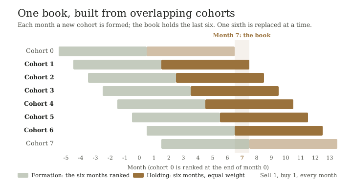
Figure 11. a construction, not market data. One sixth of the book is replaced each month, which is what makes the strategy a monthly routine rather than a twice-yearly event. The same picture reappears in the implementation section below.
The headline result is in the paper's first table. Over 1965 to 1989 the spread between winners and losers averaged 1.11 percent a month (t-statistic 4.61). In the new 1990 to 1997 window it averaged 1.01 percent (t-statistic 4.10). Across the whole 1965 to 1997 sample it was 1.09 percent (t-statistic 5.65). The authors report that the t-statistic of the 1993 paper was 3.07; the new figure is larger mainly because excluding stocks priced below five dollars reduced the variability of the spread, not because the profit grew.
Proposition JT1If n independent tests are run and the best one is reported, the probability that its t-statistic reaches t₀ under no edge is 1 − (1 − q)ⁿ, where q = 1 − Φ(t₀).
Assumptions. Each of n independent tests produces a statistic that is approximately standard normal when there is no edge. The tests are independent, which is a strong assumption; correlated tests would need numerical work.
Demonstration. The best statistic stays below t₀ only if every one of the n statistics does. Each does with probability Φ(t₀) = 1 − q, so all of them do with probability (1 − q)ⁿ. The complement is the claim. ∎
The paper applies this to its own 1993 statistic, t = 3.07, for which q ≈ 0.00107. Read as a single experiment, n = 1, the probability of a statistic this large under no edge is 0.11 percent. If a hundred independent strategies were tried in the same period and the best one reported, it becomes 10.2 percent. At 650 independent strategies it is 50.2 percent, so the evidence is no better than a coin flip when about 647 strategies were tried. The authors note that the answer depends on the reader's prior about how many tests were quietly run and discarded.
This is why the 1990 to 1997 window matters. A fresh sample cannot be searched by the same people who found the original result, so n falls toward one and the same t-statistic becomes informative again. Note the limit: the 1993 paper appeared in March 1993, so the first three years of the 1990 to 1997 window overlap the period in which it could have been read. The window is out of the original data, not entirely out of the original publication. The chapter on statistical inference treats the general problem of searched families; the usefulness verdict at the end of this chapter records how the same logic applies to a rule you test yourself.
Proposition JT2A spread with mean μ and monthly standard deviation σ reaches an expected t-statistic of t after T = (tσ/μ)² months.
Assumptions. Monthly spreads are independent with the same mean and standard deviation, so the t-statistic of the sample mean is approximately μ√T/σ.
Demonstration. The standard error of the mean of T observations is σ/√T. Dividing the mean by it gives t = μ√T/σ. Solving for T gives the claim. ∎
The paper reports means and t-statistics, not standard deviations, but the two determine σ under the assumptions above: σ = μ√T/t. For the whole sample, μ = 1.09 and t = 5.65 over 396 months imply σ ≈ 3.84 percent a month. The same arithmetic applied to 1965 to 1989 gives 4.17 percent, and to 1990 to 1997 gives 2.41 percent. These are implied figures, not reported ones. They also imply an annualized Sharpe ratio of t/√years = 5.65/√33 ≈ 0.98, gross of costs and in sample.
Two things follow. First, a true spread of 1.09 percent with σ = 3.84 percent needs about 50 months of data before its expected t-statistic reaches 2 and about 112 months to reach 3. In twelve months the expected t-statistic is 0.98: a full year of live results cannot distinguish this edge from nothing. Second, the eight years of 1990 to 1997, at 96 months, were about enough to see the edge at all, which is why the authors needed them.
The 1990s evidence
The authors ran their replication on the new window and repeated the January check that the 1993 paper had flagged. The table is reproduced from the paper's Tables 1 and 2.
| Winner minus loser, % per month | 1965–89 | 1990–97 | 1965–97 |
|---|---|---|---|
| All months | 1.11 (t = 4.61) | 1.01 (t = 4.10) | 1.09 (t = 5.65) |
| January | −2.92 | −1.21 | −2.51 |
| February to December | 1.47 | 1.20 | 1.41 |
| Share of months with a positive spread, January | 28% | 25% | 27% |
| Share of months with a positive spread, February to December | 71% | 72% | 71% |
In the 1990s the intermediate deciles were no longer strictly ordered, which the authors attribute to eight years being too few to measure small differences. Over the full sample the ordering is monotonic, from 1.67 percent a month for the winners to 0.58 percent for the losers. The January pattern is the most practically important line in the table: the spread is negative in January in every sample and was positive in only two of the eight Januarys from 1990 to 1997. If stocks priced below five dollars are included, the January spread in the full sample is −6.49 percent, which is why the screen matters.
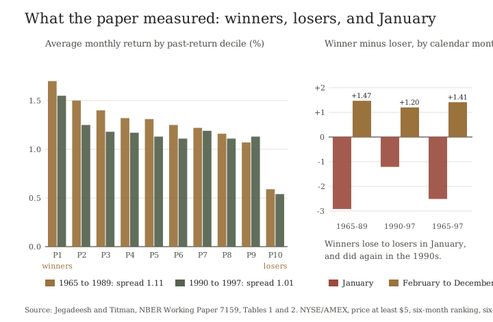
Figure 12. values printed in the paper's Tables 1 and 2. Both samples show the same staircase and the same January reversal.
Proposition JT3With weights proportional to the previous period's return less the cross-sectional mean, the expected profit equals the cross-sectional variance of expected returns plus the average own-autocovariance minus an average cross-serial covariance.
Assumptions. Returns are rᵢₜ = μᵢ + uᵢₜ with constant expected return μᵢ and E[uᵢₜ] = 0. There are N stocks. At time t each is held with weight wᵢ = (rᵢ,ₜ₋₁ − r̄ₜ₋₁)/N, so the weights sum to zero. The profit is πₜ = Σ wᵢ rᵢₜ.
Demonstration. Substitute rᵢₜ = μᵢ + uᵢₜ and r̄ₜ₋₁ = μ̄ + ūₜ₋₁. Then πₜ = (1/N) Σ (μᵢ − μ̄ + uᵢ,ₜ₋₁ − ūₜ₋₁)(μᵢ + uᵢₜ). Take expectations. Terms with a single u vanish. The deterministic term is (1/N) Σ (μᵢ − μ̄)μᵢ = σ²_μ, the cross-sectional variance of expected returns. The term in uᵢ,ₜ₋₁uᵢₜ averages to the mean own-autocovariance γ̄ = (1/N) Σ Cov(uᵢ,ₜ₋₁, uᵢₜ). The term in ūₜ₋₁uᵢₜ gives −(1/N²) Σᵢ Σⱼ Cov(uⱼ,ₜ₋₁, uᵢₜ). Adding the three gives the claim. ∎
The first term is the one Conrad and Kaul stressed: a market in which stocks simply have different constant average returns will pay a momentum rule even if no return ever predicts any other, because the past winners are disproportionately the high-mean stocks. This is the decomposition of Lo and MacKinlay (1990) that the paper uses, and it is the reason a positive momentum profit does not by itself show that past returns predict future returns.
The decomposition can be checked without any market data. The companion simulates fifty years of a synthetic market with known parameters and compares the simulated mean profit with the formula. Figures are per period.
| Own autocorrelation φ | σ_μ | Simulated profit | Formula |
|---|---|---|---|
| 0 | 0 | 0.0000 | 0.0000 |
| 0 | 0.02 | 0.0004 | 0.0004 |
| 0.1 | 0 | 0.0002 | 0.0002 |
| 0.1 | 0.02 | 0.0006 | 0.0006 |
Synthetic data, 60 independent stocks. The second row is the Conrad and Kaul world: no serial dependence at all, and a positive profit.
The authors need a test that can tell the first term from the second. That test is the subject of the next proposition.
Proposition JT4If stocks differ only in constant expected returns, the winner-minus-loser spread in every later month has the same expectation, so a one-percent monthly spread would accumulate to about sixty percent by month sixty.
Assumptions. Returns are as in JT3. Portfolios are formed from past realized returns and then followed.
Demonstration. Under constant expected returns, E[rᵢ,ₜ₊ₖ] = μᵢ for every k ≥ 1. The winners are a set of stocks chosen once, and their expected returns in each later month are the same μᵢ. So the expected spread is the same in month 1, month 13, month 37 and month 60. Summing sixty equal months of roughly one percent gives about sixty percent. ∎
Underreaction predicts something different: profits stop after the market has absorbed the information, so the cumulative line goes flat. Delayed overreaction predicts a third thing: profits reverse as prices return to fundamentals, so the line falls. The three predictions are the three lines on the left of the figure.
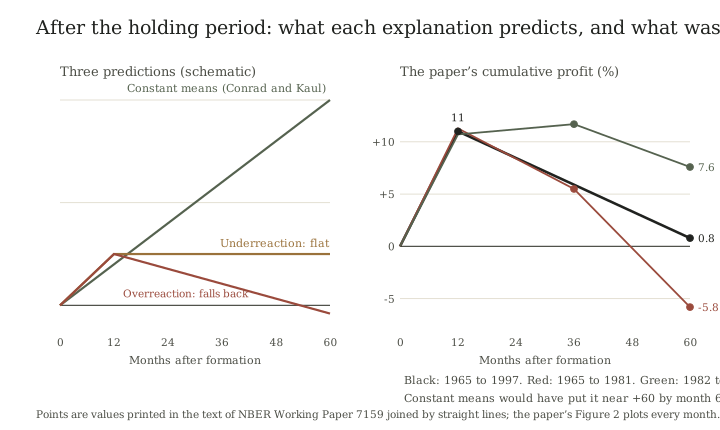
Figure 13. left, a schematic. Right, the values printed in the text of the paper, joined by straight lines; the paper's own chart plots every month.
What the authors found is in their Table 5. The average spread by year after formation, with t-statistics in parentheses, together with the Fama–French three-factor alphas:
| Year after formation | 1 | 2 | 3 | 4 | 5 |
|---|---|---|---|---|---|
| Raw spread, % per month | 0.93 (6.12) | −0.14 (−1.34) | −0.10 (−1.11) | −0.29 (−2.51) | −0.39 (−3.10) |
| Three-factor alpha | 1.09 (7.16) | 0.07 (0.76) | 0.07 (0.79) | −0.22 (−2.67) | −0.31 (−3.56) |
| January raw spread | −2.20 | −2.53 | −1.63 | −0.90 | −0.91 |
Cumulative profit climbs to about 11 percent at month 12 and falls back to 0.79 percent by month 60, according to the paper: nearly all of the first year's profit is given back over the next four. The five annual averages above cumulate to about 0.1 percent at month 60, a gap of under one point from the paper's figure that rounding alone does not explain and that the paper does not account for. Neither number is near sixty. The constant-means account cannot be the complete explanation of momentum, and the paper's F-statistic of 6.86 rejects zero profits in years two to five jointly.
The caveats are the valuable part. The authors list them and the list should be kept with the result. (1) There is no evidence of reversal in years two and three: the three-factor alphas there are positive and insignificant. The reversal is in years four and five. (2) A large part of the raw reversal falls in January, while the holding-period profit is entirely a non-January phenomenon. (3) Reversal is much weaker in the second half of the sample: in 1965 to 1981 the cumulative profit falls from 11.28 percent at month 12 to 5.49 at month 36 and to −5.81 at month 60; in 1982 to 1997 it goes from 10.71 to 11.69 to 7.59. The momentum profit in the first year is about the same in both halves (0.94 and 0.92 percent a month), so the later period differs in what happened afterwards, not in what momentum paid. (4) The size factor averaged 0.53 percent a month from 1965 to 1981 and −0.10 percent after, which the authors say accounts for part of the difference.
So the paper supports the behavioral story, and the authors ask for caution in reading it. For a trader the practical content is narrower. The profit sits in the six to twelve months after ranking. The evidence for holding the winners longer is negative, and the evidence for a big payoff from waiting for the reversal is weak, late and partly a January event.
Proposition JT5If winners load less than losers on each priced factor and each factor has a positive average return, risk adjustment raises the winner-minus-loser spread.
Assumptions. The alpha of a portfolio is its mean return minus Σ βₖλₖ, where βₖ is its loading on factor k and λₖ that factor's average return. The spread alpha is the difference of the two portfolios' alphas.
Demonstration. Subtracting the loser alpha from the winner alpha gives spread alpha = raw spread − Σ (β_W,k − β_L,k) λₖ. If every (β_W,k − β_L,k) is negative and every λₖ is positive the subtracted sum is negative, so the spread alpha exceeds the raw spread. ∎
The paper's Table 3 gives loadings on the market, size and book-to-market factors for the winner-minus-loser portfolio of −0.06, −0.29 and −0.19. Table 5's factor means are 0.49, 0.22 and 0.43 percent a month. The adjustment is 0.06 × 0.49 + 0.29 × 0.22 + 0.19 × 0.43 ≈ 0.17 points, so the prediction is 1.09 + 0.17 = 1.27 percent. The paper reports 1.29 (t-statistic 7.78); the CAPM alpha is 1.11 (t = 4.59). The winners are larger and less distressed than the losers, so the standard risk adjustments make the profit larger, not smaller.
Table 4 also splits the spread by side. The three-factor alpha of the winner portfolio is 0.30 percent a month and that of the loser portfolio is −0.99. By this measure about three quarters of the alpha spread comes from the short side (0.99 of 1.29). A long-only version is a different strategy with a different expected result, and the paper does not report it.
Proposition JT6Resampling each stock's own returns with replacement reproduces the cross-section of sample means, which includes estimation noise of about σ²/T; resampling without replacement removes that noise.
Assumptions. Each of N stocks has T per-period returns that are serially independent, with variance σ² and true mean μᵢ. The profit is the weighted-relative-strength profit of JT3.
Demonstration. The sample mean of stock i is μ̂ᵢ = μᵢ + εᵢ with Var(εᵢ) = σ²/T. Across stocks the variance of the μ̂ᵢ is σ²_μ + σ²/T, because the noise is independent of the true mean. Resampling with replacement from a stock's own returns draws i.i.d. observations whose mean, conditional on the sample, is exactly μ̂ᵢ. By JT3 with no serial dependence the profit is then the cross-sectional variance of those means, σ²_μ + σ²/T. A permutation keeps the same values, so its cross-sectional variance of means is the same, but the draws are no longer independent, which subtracts about σ²/(T − 1) per stock and cancels the noise term to first order. ∎
This restates, in terms of estimation noise, the mechanism the paper gives in its Appendix, which describes the same bias as one extreme observation being drawn into both the ranking and holding periods. The paper's Table 8 reports what it does to Conrad and Kaul's experiment.
| Simulated weighted-relative-strength profit | Profit | Share of actual |
|---|---|---|
| Actual data, 1965–97 | 0.00380 | |
| Resampled with replacement | 0.00410 | 107.89% |
| Resampled without replacement | 0.00002 | 0.53% |
The authors conclude that the with-replacement result came from the bias and that very little of momentum comes from differences in constant expected returns. Their later Review of Financial Studies article describes a variant of the bootstrap that it says it shows analytically to be unbiased. The companion reproduces the mechanism on synthetic returns, where the truth is known.
| Synthetic world (200 stocks, T = 10, σ = 0.25) | True profit | With replacement | Without replacement |
|---|---|---|---|
| No true dispersion in means | 0.0000 | 0.0059 | 0.0002 |
| True σ_μ = 0.06 | 0.0037 | 0.0095 | 0.0038 |
The noise term σ²/T = 0.0063 predicts the with-replacement excess, and the permutation recovers the true figure within sampling error. The paper's Table 6 makes the related point directly: the cross-sectional variance of sample mean returns is 134 percent of the profit to be explained. A quantity that measures the wrong thing more than fully can explain the profit, which is how it got to explain all of it.
How to run it: the six-month strategy, step by step
Everything above is analysis. This section is a procedure. It is written as a specification, in the sense the blueprints chapter uses the word: a set of decisions to be fixed before the first trade and a set of tests to be run afterwards. It does not say the strategy will work for you, and the authors of the paper do not say so either.
The specification
The left column is what the paper did. The right column is what you must decide and write down.
| Item | The paper | Your decision, fixed in advance |
|---|---|---|
| Universe | NYSE and AMEX stocks; NASDAQ excluded | A point-in-time list that includes stocks that later delisted |
| Price screen | At least $5 when the holding period begins | The same, plus a liquidity floor of your own |
| Score | Compounded return over the last six months | The same. A different lookback or a skipped month is a different strategy |
| Groups | Ten groups of equal size | Ten, or fewer if the universe is small |
| Weights | Equal within each group | Equal, with a cap per name |
| Holding | Six months, in monthly overlapping cohorts | The same: replace one sixth each month |
| Sides | The spread, winners minus losers | Long-short, or long only: a different strategy |
| Costs | None modeled | A written cost, borrow and impact model |
| January | Reported separately, not special-cased | A rule fixed in advance: trade, lighten or pause |
| Risk scaling | None | Fixed in advance; chapter 18 gives the crash evidence |
The monthly routine
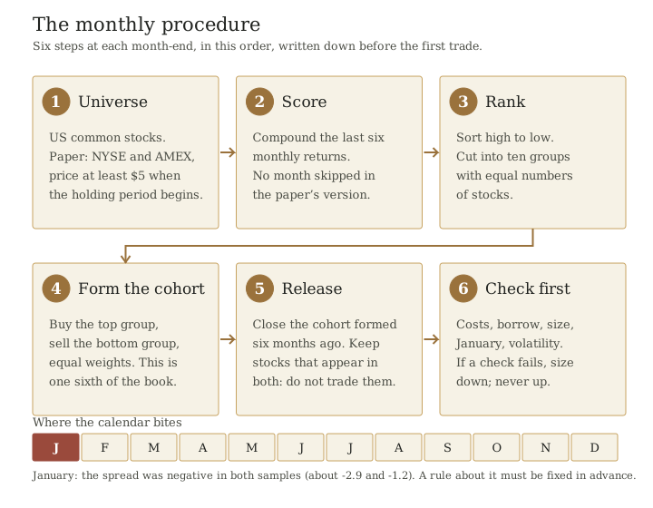
Figure 14. a construction. The order matters: the checks in step six come before the orders, not after the loss.
- Fix the universe. List every eligible stock as of the month-end, including names that will later disappear. A list built from today's survivors will flatter any backtest and is not a point-in-time record.
- Score. For each stock, compound its last six monthly returns. A stock with fewer than six months of history is ineligible.
- Rank and cut. Sort from best to worst. The top tenth of the list is the winners and the bottom tenth is the losers.
- Form the cohort. Buy the winners and sell the losers short, equal weights, in an amount equal to one sixth of the target book. Record the date, the names and the amounts.
- Release. Close the cohort formed six months earlier. A stock that appears in both the old and new cohort can be left alone: trade only the difference.
- Check, then send. Before orders go out, confirm that costs, borrow availability, position limits, the January rule and any volatility scaling allow the trade. If a check fails, reduce the size. Do not increase it.
One book from six cohorts
Because one sixth of the book turns over each month, the book needs six months to fill. Cohort 0 is ranked at the end of month 0 and held during months 1 to 6. Cohort 5 is ranked at the end of month 5 and held during months 6 to 11. So month 6 is the first month in which all six cohorts are held.
| Month-end | Action | Fraction of the target book invested during the next month |
|---|---|---|
| 0 | Form cohort 0 | 1/6 |
| 1 | Form cohort 1 | 2/6 |
| 2 | Form cohort 2 | 3/6 |
| 3 | Form cohort 3 | 4/6 |
| 4 | Form cohort 4 | 5/6 |
| 5 | Form cohort 5 | 6/6 |
| 6 | Release cohort 0, form cohort 6 | 6/6 |
Every month after the fifth is a sale of the oldest cohort and a purchase of the newest. A run of paper trading through these first six months costs nothing, and it is the cheapest way to find errors in the data and the record-keeping.
Proposition JT7If one sixth of each leg is replaced every month, gross traded notional is at most four times each leg per year, and a long-short book breaks even at a one-way cost of 12μ/8 per dollar traded.
Assumptions. Every cohort is bought once and sold once, at equal weight and no netting across cohorts. The monthly spread is μ, taken as a simple sum of twelve months. Costs are paid at a fixed rate c per dollar on each purchase and each sale.
Demonstration. A leg holds six cohorts each of weight 1/6. Each month one cohort is sold and one bought, each of weight 1/6. Over twelve months that is 12 × 1/6 = 2 purchases and 2 sales of the whole leg, a traded notional of 4. The book has two legs, so 8 in all. Net annual spread is 12μ − 8c. It is zero when c = 12μ/8 = 1.5μ. ∎
The figure of four is an upper bound. When a stock stays in the top group in consecutive months it sits in several cohorts at once, and the combined book does not need to sell and rebuy it. With μ = 1.09 percent a month, 12μ = 13.08 percent a year. At a one-way cost of 10 basis points the net figure is 12.28; at 50 basis points it is 9.08; and it reaches zero at 163.5 basis points a side.
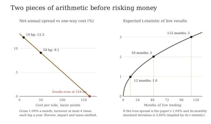
Figure 15. arithmetic on the paper's gross figures, not a forecast. It omits borrow fees, market impact, taxes and the usual shrinkage of published results.
The left panel is deliberately generous. The paper's gross spread is the most favorable number in this chapter, and it is a gross number. The right panel is the harder one. It says that even when the spread is exactly what the paper reports, twelve months of live results give an expected t-statistic of about one, and about fifty months are needed before two. The table gives the same arithmetic as uncertainty in the estimated monthly spread, using the implied σ = 3.84 percent.
| Months of live results | Standard error of the mean spread (points a month) | About 95% band around the estimate |
|---|---|---|
| 12 | 1.11 | ±2.2 |
| 24 | 0.78 | ±1.5 |
| 50 | 0.54 | ±1.1 |
| 112 | 0.36 | ±0.7 |
After a year, the band around the average monthly spread is twice as wide as the spread itself. A drawdown or a good quarter says almost nothing about whether the rule works. That is why the retirement rule belongs in the specification, before the first trade.
A reference implementation
The companion contains a small, tested implementation of the ranking, the cohorts and the overlapping book. It is standard-library Python. It is for checking your own understanding of the procedure against synthetic data, and it is not connected to any broker or data feed.
from momentum_paper import formation_ranks, decile_members, momentum_spread_series

# history[stock][month]  = that month's return
# start_price[stock]     = price when the holding period begins
ranked = formation_ranks(history, month, lookback=6, min_price=5.0, next_prices=start_price)
winners, losers = decile_members(ranked)          # top tenth and bottom tenth
cohort = {'formed': month, 'long': winners, 'short': losers}

# The book is the last six cohorts; the oldest is released each month.
book = (book + [cohort])[-6:]

# Research use: the monthly winner-minus-loser series for a whole history.
series = momentum_spread_series(history, range(6, last_month), lookback=6, hold=6)
The test suite plants a persistent drift in a synthetic market and confirms the function finds a spread, then removes it and confirms the spread vanishes. It also checks that the price screen looks at the start of the holding period, that a stock with missing history is ineligible, and that the book is not fully populated until six cohorts exist. It has not been run on real data.
What changes if you shrink it
Suppose the eligible universe is 1,200 stocks and the book is 1.2 million dollars on each side. The top group is 120 stocks. One cohort is 200,000 dollars, or about 1,667 dollars a name, and at steady state the long leg can hold up to 720 positions. That is a large and expensive book for a small account, and most people will reduce it. Every reduction changes the object and none of the changes is measured here.
- Fewer names. Quintiles instead of deciles, or a large-cap universe. The spread is diluted and its variance rises with fewer names, which lengthens the 50 months needed to see it.
- Long only. About a quarter of the paper's alpha spread came from the winners. See JT5.
- Shorter holding. More turnover per unit of spread, so the cost line in the figure steepens.
- A fund or an index product. A fund that advertises momentum has its own rules, costs and rebalance dates. It is not the paper's strategy.
The card to write before the first trade
| Decision | Example entry |
|---|---|
| Question | Does the six-month winner-minus-loser spread net of my costs stay above zero? |
| Specification | The table above, with the right-hand column completed |
| Cost model | Spread plus commission per side, borrow fee on the short leg, and an impact allowance, each as a number |
| Evidence status | Research and paper trading: no money until the record and data pipeline have run cleanly for six months |
| Earliest meaningful test | 50 months, at which a true spread of the paper's size has an expected t-statistic of 2 |
| January rule | One of: trade as normal, halve size, or pause for the month. Fixed now, not after the first bad January |
| Retirement rule | A number of standard errors below the expected spread, and a date, stated before the start |
| What will not change the plan | A single drawdown, a good quarter or a story in the news |
What came after the paper
The paper's 1990 to 1997 window has since been followed by a long record, which this edition covers elsewhere: momentum crashes in panic rebounds, and volatility-scaled versions that reduce them (chapter 18); average declines of returns after publication across many anomalies (chapter 6); and time-series momentum, which is a different object (chapter 47).
Two later papers on costs disagree, and the disagreement is informative. Korajczyk and Sadka (2004), using intraday data to estimate proportional and price-impact costs, report that liquidity-weighted and hybrid momentum strategies could absorb several billion dollars before the apparent profit vanished. Lesmond, Schill and Zhou (2004) report that standard relative-strength strategies require frequent trading in disproportionately high-cost securities, and that the stocks generating large momentum returns are precisely the high-cost ones. This edition read both only in summary. The difference between them is partly in how the strategy is constructed, which is the point of the specification table: the paper's gross spread does not come with a cost, and the cost depends on choices made in steps one to six.
Usefulness verdict
What the paper establishes, as reported. In U.S. stocks from 1965 to 1997, buying the past six months' winners and selling the losers earned roughly one percent a month gross, about the same in a later window; the profit was not explained by the market, size or value factors; and the profit reversed over the next four to five years, mostly late and partly in January. The explanation from constant differences in expected returns does not fit.
What it does not establish. The paper does not show that the profit survives costs, borrow, taxes or capacity; does not say what happens in any other market or era; and does not distinguish cleanly between underreaction and delayed overreaction. It cannot show that a strategy published in 1993 still works.
What you can use today. The paper is most useful as a set of questions to put to your own rule. How many versions did you try before this one (JT1)? How many months of live data will you need (JT2)? Does the result disappear in a second period, or in January, or beyond the holding window (JT4)? Does risk adjustment raise it or lower it (JT5)? Is the test you are running immune to its own measurement noise (JT6)? What does turnover cost (JT7)? And the implementation section is a template for writing down the answers before the money goes in.
Source notes
JT1 to JT7 are original demonstrations in this edition, derived from the assumptions stated in each. The decomposition in JT3 is that of Lo and MacKinlay (1990), as used in the paper. The implied standard deviation, Sharpe ratio and months-to-detect in JT2 and the cost arithmetic in JT7 are this edition's calculations from the paper's published means and t-statistics; the paper does not report them. The synthetic simulations are in books/research/momentum_paper.py, tested by tests/test_momentum_paper.py.
Empirical claims are drawn, with the figures as stated by their authors, from: Jegadeesh and Titman (2001), Journal of Finance 56(2), 699 to 720, doi:10.1111/0022-1082.00342, with figures transcribed from the working-paper version, NBER Working Paper 7159 (June 1999); Jegadeesh and Titman (1993), Journal of Finance 48(1), 65 to 91; Jegadeesh and Titman (2002), “Cross-Sectional and Time-Series Determinants of Momentum Returns,” Review of Financial Studies 15(1), 143 to 157, doi:10.1093/rfs/15.1.143 (introduction read); Conrad and Kaul (1998), “An Anatomy of Trading Strategies,” Review of Financial Studies 11(3), 489 to 519; Lo and MacKinlay (1990), Review of Financial Studies 3(2), 175 to 208; Fama and French (1993), Journal of Financial Economics 33(1), 3 to 56; Korajczyk and Sadka (2004), “Are Momentum Profits Robust to Trading Costs?” Journal of Finance 59(3), 1039 to 1082, doi:10.1111/j.1540-6261.2004.00656.x (summary read); and Lesmond, Schill and Zhou (2004), “The Illusory Nature of Momentum Profits,” Journal of Financial Economics 71(2), 349 to 380, doi:10.1016/S0304-405X(03)00206-X (summary read). The paper's own cited behavioral models are Barberis, Shleifer and Vishny (1998), Daniel, Hirshleifer and Subrahmanyam (1998), and Hong and Stein (then a working paper). A record of what was read, at what depth, is in books/research/expansion/momentum-2001-sources.md.